


![Renewable Energy Sources Aktu FULL EXPLANATION [✓UNIT-4] #renewableenergysourcesaktuunit-4 #aktu](https://i.ytimg.com/vi/ojCnA9erQcE/maxresdefault.jpg)







![[MERL Seminar Series Spring 2023] A Beginner’s Guide to Quantum Sensing Illustrated with Nitrogen...](https://i.ytimg.com/vi/58dRcpcDA0Y/maxresdefault.jpg)

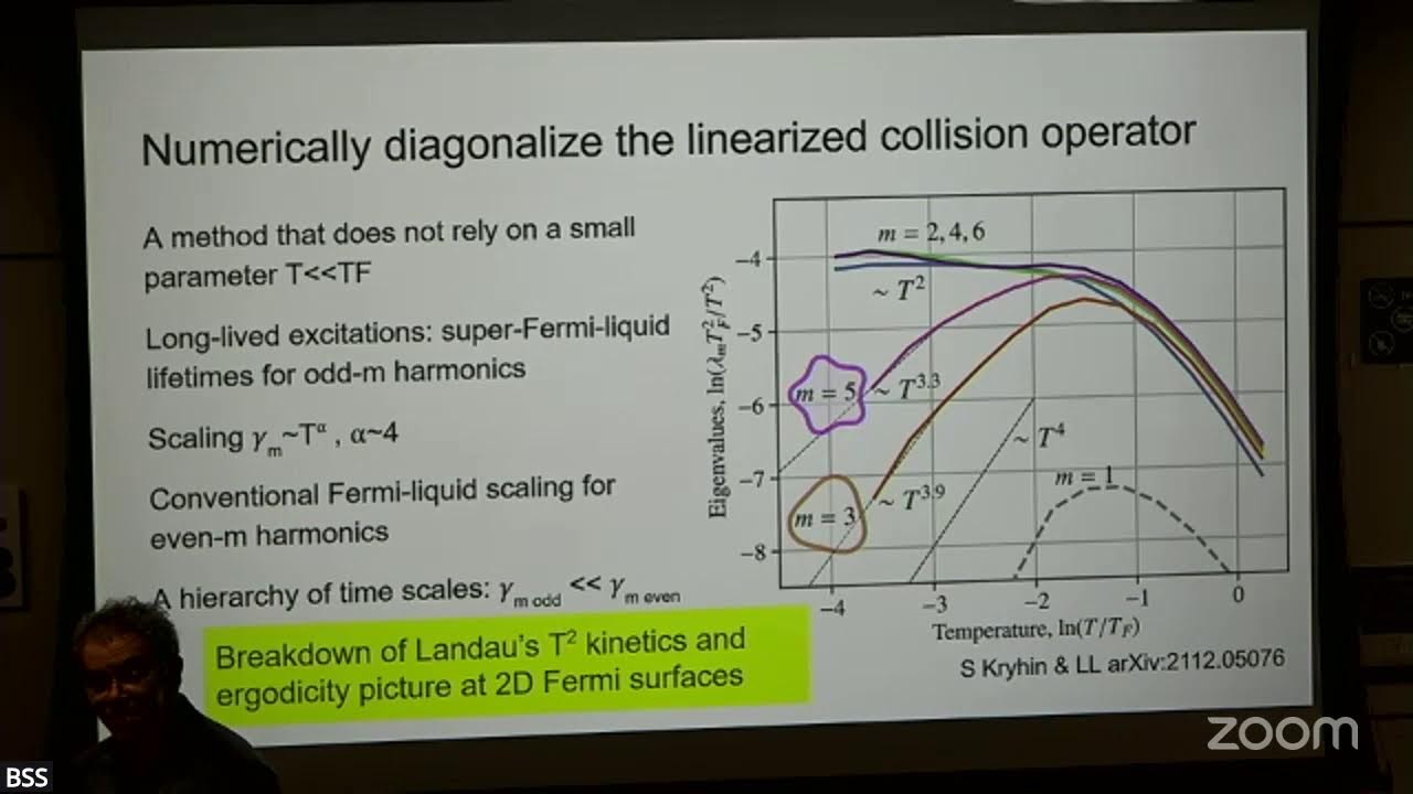



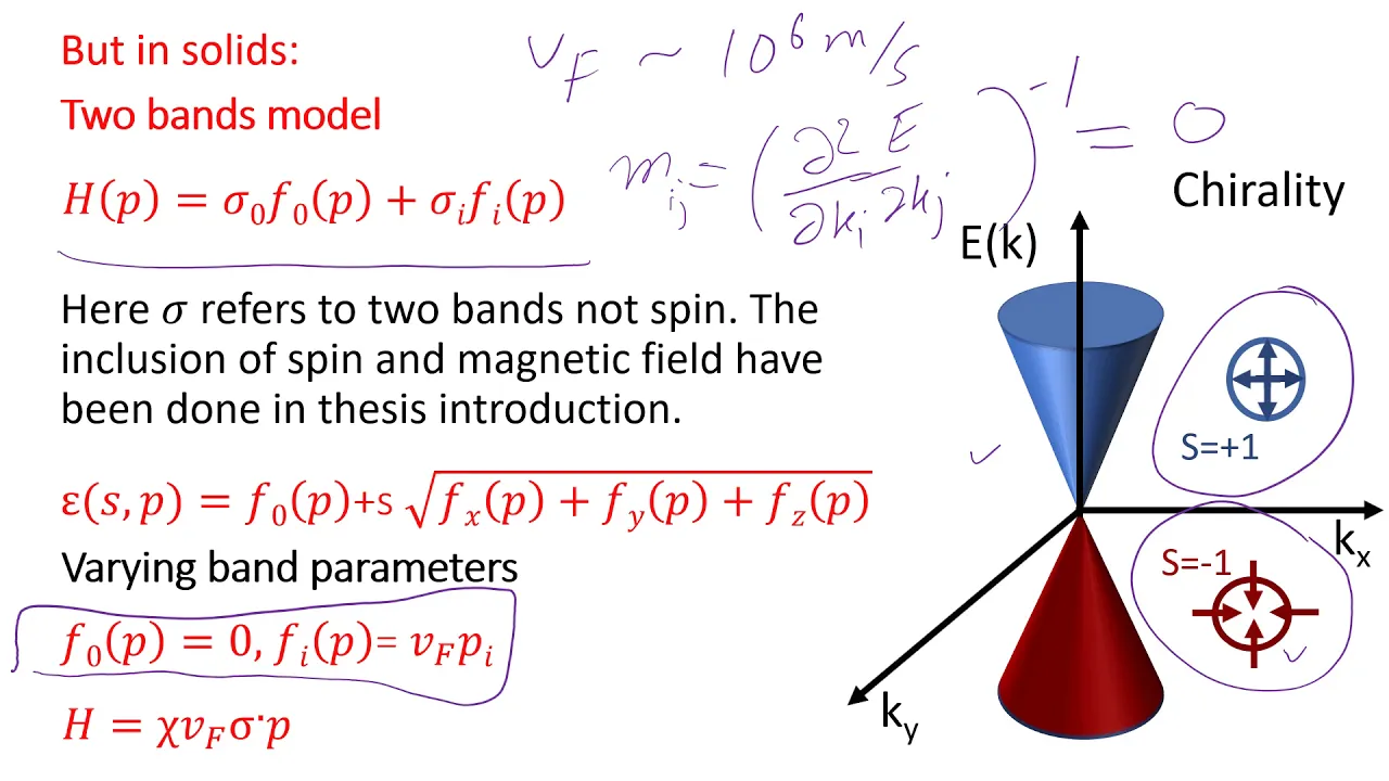





In graphene devices operating near charge neutrality, electron liquids exhibit hydrodynamic transport behavior where viscous electron flow dominates over individual electron scattering. This regime produces anomalous thermoelectric effects that violate the Wiedemann-Franz law and Matthiessen's rule, including a giant enhancement of the Lorenz number (ratio of thermal to electrical conductivity) by up to an order of magnitude. The thermal conductance shows a sensitive Lorentzian dependence on electron density, with the width determined by fluid viscosity, enabling viscosity determination through purely thermal transport measurements. In Corbino geometry, the irrotational nature of hydrodynamic flow causes forces to be expelled from the bulk, resulting in drops of both voltage and temperature at system boundaries. These phenomena arise because the absence of Galilean invariance in graphene creates qualitatively new features in thermoelectric transport, fundamentally different from conventional metals.
Hydrodynamic Thermoelectric Transport in Graphene Near Charge Neutrality
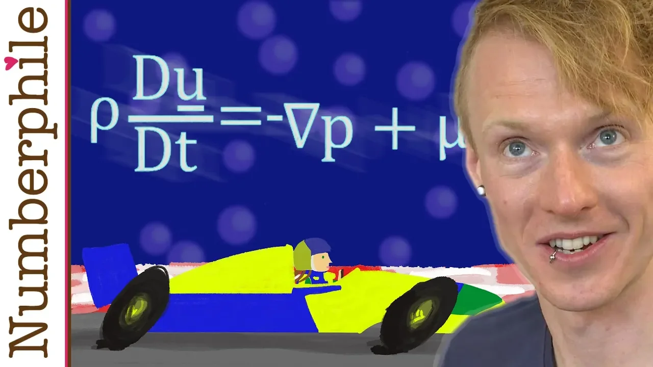
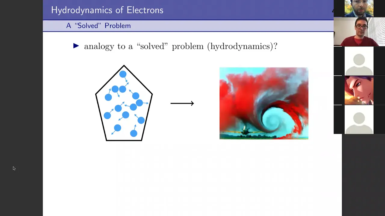
Added:awesome all right i think we're live um so today i'd like to introduce alex levchenko from university of wisconsin to give our seminar um and his talk will be about hydrodynamics thermoelectric transport near charge neutrality and with that take it away alex okay perfect thank you guys um yeah so i uh prepared for you uh a couple of slides to so let me see how do i move through presentation okay and give me one sec i'll try to do this highlighter for you um [Music] you you see that right um all right so i prepared for you a couple of sort of teasers to introduce the topic first which are examples from classical physics but they are i think very beautiful examples maybe to spark your curiosity a little bit uh then we'll go to some more specific introductions few topics of aerodynamics in the context of electron liquids and then the bulk of the presentation would be a bit more technical uh technical matter so when i speak about these topics to students i typically start with this slide um and this slide gives you a screenshot from the clay institute of mathematics uh and specifically the page which is devoted to millennium problems you probably know that these problems are uh give you a grand prize of one million dollars if you solve them and so the this problem of navier stocks is currently unsolved uh and they say that although and navier stocks equations were written down in 19th century our understanding of them remains minimal and the challenge is to take substantial progress towards the mathematical theory which would unlock the secrets hidden in obvious stocks equations so you need to click uh on this link here for the official problem description and i wish you uh best of luck uh now uh when you read it uh it's sort of very interesting how mathematicians view these topics i don't think that for physicists the concept of navier stokes equation would sort of resonate as something fundamental after all we understand that these equations are certain approximations for certain things uh but a couple of examples that i prepared for you uh would sort of reinforce this thinking that indeed there are lots of very interesting things that are hidden in them uh even at the classical level that are quite surprising so in order to stimulate that uh sort of discussion uh so let me show you one fact and then to uh to show you an example so one thing which is written in all of the textbooks and one of the first things you sort of see in here dynamics is the stocks formula and stocks himself made lots of contributions to aerodynamics so he derived an equation for the drug force of an object moving through a viscous fluid saying that if this velocity of the object v is small enough then the force is some coefficient radius of the sphere times the viscosity of the fluid and sort of fun fact about this uh formula that sort of transparent but maybe not so uh maybe not immediately known to you is the following so if we disregard this numerical coefficient for a second and we'll do a small trick we will multiply this equation by extra power of viscosity so we have viscosity squared over viscosity and then we multiply and divide by the um mass density of the fluid then we will be able to form this dimensionless coefficient a which is a typical size of the object for the sphere would be radius v row over eta and this should resemble to you uh reynolds number uh and then will be ratio viscosity squared over the mass density and so the nice feature of this formula is that if you'd like to drag an object through a viscous fluid any object of any size but you'd like to drag it in such a way as the rayleigh's number is one then the force that you need to apply sort of universal and is the property of the fluid itself so it's just the viscosity squared over the mass density and for water it is ten to the power minus four dens so it means that let's say dragging a big ship or dragging a tiny piece through water would require the same force as long as you drag it the trend is number one all right so other thing that is a bit uh more curious um is the so-called scale-up theorem uh you can find a very beautiful discussion of this thing in a very famous uh article by purcell which is published in the american journal of physics if you haven't seen this article i strongly advise it's really fun reading almost like a bedtime story but it's really beautiful and field of stories and ideas and so he talks about the following he talks about life at extremely low reynolds numbers when in the navies toxic equation that is just sort of a newtonian equation of motion for the fluid uh if we have an extremely viscous regime inertia term is not relevant convective term which is non-linear in velocity is also not relevant everything is governed by the highly uh high viscosity and there is the scallop theorem that says that if there is an object that tries to swim through extremely viscous environment having only one degrees of freedom so let's say in this case for the scallop this will be an angle of opening and let's say the scallop would like to open its shell and close the shell to do this reciprocal motion in order to swim so the statement is that this will not be possible so let me show you an actual experiment of that and so this is a fish uh in a container and so i got this light from my grecia file collection kind of appreciate it for for sharing this so let me try um so i need to undo um undo the laser pointer and try to run the video for you so you need to pay attention right now to the head of this fish this fish would open a mouth and will try to swallow one of these food pieces floating around and then it will close its mouth and see what happens so i'll run it a couple of times so it opens the mouse a little piece goes inside it closes the mouse and it escapes let's do it again opens closes okay so uh so this fish was fooled uh so the water in this container was made purposely more viscous than the normal environment to this fish and so it does a normal thing for it uh when it tries to eat but it doesn't work uh yeah and so this is kind of an example uh of this um uh sorry i'll just repeat uh example of this um uh scalab theorem uh that by just simply repeating the motion you could not you could not swim and this fish unfortunately couldn't figure it out how to solve navistox equation now in his article um purcell discusses that in order to swim you actually needed bare minimum two degrees of freedom and he discusses this really beautiful example of the swimmer doing certain cycles so let's say we have a swimmer with some initial position with let's say arms up and we do a sort of cycle by changing angles in such a way that we return at the end of the cycle to the same position then in parameter space of these angles we form a loop closed cycling can be proven that the displacement of the swimmer would be proportioned to the area enclosed uh in the cycle and that sort of starts to resonate with things like very phases and some adiabatic invariants and so on and that's all true and it's all a very beautiful connection and i at this point just simply uh make reference to beautiful work of vilcek and shafir and lebron kenneth and god who showed that uh swimming in highly viscous environment by just simply changing the shape of the swimmer uh is actually connected soon on the billion gauge theory and so on so i mean indeed there are sort of extremely beautiful examples uh in the navier stocks even in the most sort of trivial and you would say boring regime of extremely viscous flow but yet there are these jewelers that you could find and this i just live for you to enjoy and maybe i do some extra reading when you have some spare time ah so now coming to uh a topic of today's presentation about electronic aerodynamics so next few slides are introduction and this is very very condensed introduction of the research that took place about uh 60 years so have you cover many decades but i'll do it very uh quickly and i will introduce sort of more uh most important topic for us which is called the guruji effect i will talk about what it is and how this grugia effect kind of manifests in more modern examples of electronic hydrodynamics in graphene or other strongly correlated fluids so first of all um why it is sort of unusual to even think about hydrodynamics and applications to electron liquids uh so typically uh when we think about electronic transport and solid state we think of electrons scattering of impurities uh electrons getting phonons electro scattering of other possible excitations we sort of intuitively think this to be a highly quantum mechanical problem and the picture of viscous flow like water flows through the pipe is not sort of a picture that first comes to our mind uh nevertheless uh there are regimes um then this picture is actually possible and this is the regime when the length scale of momentum conserving electron electron collisions becomes the shortest length scale in the problem so when we think about a flow of i don't know oceans or coffee in a cup we are not interested about the length scales of intermolecular scattering we are looking at the much microscopic scales and so as long as we can ensure that electronic equilibration occurs at the time scales in length scales that are small enough compared to other scales at which electrons lose their momentum and energy then these genetic aerodynamic descriptions could be applicable and the power of aerodynamics is that it naturally describes most fluids regardless of the strength of interaction and some other details but it requires as an input parameter just a small set of uh input variables and this variables would be thermodynamic quantities that describe the state uh of the fluid and then also some kinetic coefficients such as viscosities so i would say that the field of electronic aerodynamics was uh pioneered by guruji uh in early 60s he worked in harika physical technical institute at that time and then he spent his professional career at the low temperature institute in kharkiv i used to leave uh two trolleybus stops from from the institute and i'm kind of intimately connected to this place uh this place uh has been in the news for unfortunate that said reasons quite a lot these days but um so all of the work on electronic aerodynamics by guruji and his group was done uh back in uh ukraine and kharkov so he uh derived an equation of motion for electron liquids in a metal that looks like very much uh as an ivia stocks equation he started however from much more microscopic description he started from quantum kinetic equation for electrons and phonons uh subject to some disorder scattering but he made this assumption that i described to you in the previous slide that electrons scatter of themselves much more efficiently than the scatter of phonons and etc so he assumed the existence of slow consort variables and he projected kinetic equations into the slow modes uh in this case slow mode would be just a hieronymic velocity of the fluid and he arrived at the end of the day much simplified description uh so there are electric field driving forces and the balancing forces are viscose stresses new here is a kinematic viscosity kinematic viscosity would be shear viscosity divided by mass density and then some term that describes that pure relaxation of electrons are scattered with impurities and then this equation should be supplemented by the constituent relation connecting the particle current or electrical current to aerodynamic velocity u now in the regime when viscosity is irrelevant for some reason let's so let's say uh very efficient so alex do you mind if i ask you a question right now yes yes so you mentioned that the uh scattering time of impurities should be much longer than the election election scheduling time that's right where is this in this equation this can we see anywhere in this formula in this equation not but it is uh it it should be appeared in much earlier level when you start with kinetic equation and the matter of fact that you have a hydrodynamic mode so in order to arrive at this equation you sort of need to consider the flow of the liquid in a reference frame that is flow so you need to apply a boost or gallium transformation so you say that let's say energy dispersion would be something times p times u and this is where you would assume that you have slow modes and proceed with this sort of projection procedure so you need a slow varying variables on certain time scales so at this level it is not present but it is present in much earlier level of the kinetic theory well but you will have it very soon on your right bottom you know picture you have led that's right correct correct i will come to that just like this so here i just want to say sort of to connect to regimes one is more standard sort of regime kinetic regime that if viscosity is irrelevant we see that you heronamic well this microscopic velocity is just proportional to relaxation time this give us current proportion to electric field and so this is ohmic regime that is governed by the druid conductivity uh however if we are in opposite regime when the there is no relaxation in the bulk of the flow and everything occurring due to the viscous stresses of course then we need to answer the question where the relaxation of momentum occurs because electron electron collisions conserve momentum unless we talk about the um clubs that are not in this picture either so then uh we need to think about the flow in a finite size geometry so let's say in a quantum wire of certain size or in the whole bar of certain width w then momentum occurs at the boundaries and there is a momentum out flux due to risk stresses occurring at the boundaries and so then this flow realizes sort of an analog of this poisson flow uh and we can derive uh and what guruji did derive this formula for conductance in this regime when conductance scales quadratically with the width of this channel and then is inversely proportional to the viscosity of the fluid now to what elia was asking me is that if you forget about the driving force meaning the left hand side of this equation and just correspond um concentrate to the right hand side we can see that this combination of the two terms introduces an intrinsic length scale in the problem so indeed uh kinematic viscosity times laplacian by dimensional units is kinematic viscosity divided by some length scale squared times u and this second term is u uh divided by tau so comparing the two we see that there is intrinsic length kiloxi that is roughly speaking uh uh kinematic viscosity divided by tau multiplied by tau excuse me in taking the square root of this expression which can be massaged into the geometrical mean between electron uh momentum relaxing electron impurity scattering and momentum conserving collecting electron scattering which is inside of the kinematic viscosity and this object is called the gurji lens and this gorgeous lens it covers the crossover between the bulk flow so meaning that if the width of this channel is much bigger than lg then you are sort of back to the ohmic regime or if the width of the channel is smaller than lg you are back into the stocks terminated regime of electronic hydrodynamics now uh if you invert uh conductivity and you write resistivity then you'll see that resistivity would be proportional to viscosity like in the stocks formula and so guruji predicted himself that if this regime is realized it should manifest itself with the negative differential resistance so it should be a regime of temperatures where you try to increase well you increase the temperature but resistance goes down now if you think about this from the mindset of sort of a conventional thinking about electronic transport this is highly counter-intuitive because we think of resistance as sort of a measure of scattering we increase temperature we increase probability of scattering of electron scattering of anything possible phonons and so on so resistance should go up but again the whole spirit here is that you shouldn't think like this you should think about this collective behavior of electron fluids and i should remind you that in fermi liquids and i will elaborate on the next slide that viscosity is inversely proportional to the square of temperature so you increase temperature viscosity goes down resistance goes down so that is in essence of the guruji effect uh from the point of view of classical physics i think this regime is very intuitive and we experience this every day when we cook so if you if we pour uh oil in a frying pan and we heat up the oil it becomes more fluid-like so resistivity this drug goes down because the fluid viscosity decreases with an increase of temperature ah so now so pay attention this is 63 he wrote a review article that was published in the physics suspected uh which is russian review journal about the same time and i would say that was it uh and then next i would say big development was in 1994 because it took that much time sort of to to get into the regime that this becomes reality rather than uh sort of theoretical desire to get into uh materials that are pure enough and tunable enough that you can realize it and this experiment from lawrence modern cup is considered to be like a first uh hint into the electronic aerodynamics it is not really a linear response measurement so he was using current to inject into the quantum wires into dax to locally heat electrons by joule heating and he plot he measured differential non-linear resistance and he thought about the current has effectively been effective electronic temperature as i said through the dual heating mechanism but he saw this downturn in resistances and attributed this as a manifestation of the heronic behavior as you can see even at the title of the paper itself again i would say that the field was quiet for quite some time even after that i couldn't find much of the discussion of electronic aerodynamics really and i would say the next milestone uh sort of appeared with the discovery of very clean high mobility uh two decks and graphene and so here i collected few representative plots of now linear resistant measurements uh of a variety of 2d systems as a function of temperature so some of these plots i took from a very beautiful and nice uh review by boris pivak sergey kravchenko steve kivelson and huang gao uh un strongly correlated to this electron and whole systems so as you can see uh these are holes of this upper plot are holes in gallium arsenide quantum wells exhibiting this behavior of uh non-monotonic temperature dependence of resistance in in that study which is also co-authored by hong kong uh their statement is that they believe that this is intrinsic electronic effect because if you try to think about phonon contribution it's out of the picture uh also pay attention to the scale of temperatures these are in the range of small uh temperature uh regime you of course can ask me how this could be attributed to electronic hydrodynamics that sort of is a higher temperature regime we need to ensure that electron electron meaning three pass is small but i need to remind you that in regime of very low densities fermi energy itself could be as small as one kelvin or 10 kelvin so so even though by actual numbers it looks like very low temperature think you always need to compare it to an actual fermi energy in the systems and for this systems they are also highly correlated typical rs parameter which measures the strength of electron interactions would be somewhere in the range of 10 to 30 to even 40 so some of the systems are the onset of the wigner crystallization in 2d so they're highly correlated so 2d holes in silicon mosfet 3d holes and pdop silicone germanium and this plot here in the lower right side i took from a reasonable sort of first experiment from pablo on magic angle twisted by layer graphene this transport measurement was done in a normal state just above this onset of all of this cascade phase transition superconducting and insulating behavior this is normal state measurement uh in the in the panels represent the density of 2d system this is zero field measurement as a function of temperature and again you see this upturned downturn upturn the monotonic behavior which is uh having this down turn slope reminiscent of the earlier proposal of gurjee saying that perhaps this is uh should be attributed to a collective viscous behavior of electing liquids so my goal is maybe not so much to convince you that this is exactly the case but i will try to give you hopefully plausible and convincing argument that maybe this is indeed the case and so let me try to do that so i will do that first by giving you example from 1d physics it's just much easier to try to give you this convincing argument but this can be generalized to 2d and i will continue to elaborate in the next slice on this so imagine that we will consider a flow of electrons strongly interacting electrons in 1d channel let's assume that for kind of realistic also discussion that this 1d channel electron liquid is subject to a long grange uh in homogeneity potential not short-range impurities but long range of potential due to let's say doping layer or some uneven screening that creates a prop profile of up and down of local value of electrochemical potential so let's consider the flow so what would be microscopic description of such fluid so we need to ensure continuity equation and i will consider only steady state properties and then the navier stocks steady statement via stocks and the linear response would be simply a balance of the risk stresses and external driving this pressure return by general thermodynamic arguments can be written as the density times gradient of the local chemical potential times entropy and gradient of temperature and the chemical potential and electric field can be driven into a general emf so we will consider the response of the system to uh external electric field now uh the continuity equation tells us that the current which is given by velocity times particle density is constant so we need to ensure that the gradient is zero nevertheless density and current individually can be of course coordinate dependent depending on the cross section when i stand in this wire now then i take this velocity and bring into the stress tensor uh in 1d there is no shear there is only bulk flow so uh stress tender will be just the bulk viscosity times the divergence of this velocity field so the stress tensor would be given by uh bulk viscosity current and gradient of inverse density and then i ignoring the stress i can calculate uh with the help of six volume of landau lifts and fluid dynamics i can calculate entropy production in this viscous flow which is the average of the viscous stress was uh basically the gradients of the velocity which roughly speaking just square of this expression so i will get current squared viscosity and then averaged over the space gradient of inverse density and then i can compare this to the joule heating um in the flow and this gives me already resistance so this part will give me a resistance which is of viscous origin but entropy production is also possible due to heat fluxes and i need to do the same type exercise with the second equation for the entropy current and believe me that similar line of considerations will give you a second contribution to resistance that would be inversely proportional to thermal conductivity so in 1d resistance is conductance quantum temperature divided by thermal conductivity multiplied by entropy per particle squared and then second term is bulk viscosity times the gradient of inverse density squared now in 2d there will be a factor of two here in the overall pre-factor and the third second term which is viscous term should be generalized you need to add additive contribution from the shear viscosity here now the power of the prediction of this formula is that nowhere in this derivation we said anything about the strength of interactions or being perturbative in nature of sort of which is hinted in all of the let's say boltzmann calculations all details of inter-particle interactions are hidden in this quantities meaning the thermal conductivity viscosity equation of state which is in this case is given by entropy density and so on so of course we could not reliably calculate them in a strongly correlated fluid but generality and power of aerodynamics is that if they are given to you let's say from the measurement then you can use them to make predictions for other quantities in this case for resistance so let's try to analyze this quick question so the angular brackets what's the averaging averaging over the space so it's uh so it's it's highlighted here so it's it's it's not uniform due to this uh potential right correct yes okay yeah so i just tried to make it a little more realistic for actual samples and i will show you the stm data in 2g graphene of course shows that the system is none homogeneous and so this would actually lead us to new hydrodynamic features that i will discuss maybe in 15 minutes from now so now what i'd like to do is as a sort of a poor theorist try to distill certain predictions from this formula for some states that we know and at least qualitatively so let's analyze this formula for a 2d case let's try to do that and i will do this for a fermi liquid regime where we will take some fermi liquid expressions for thermal conductivity and in discussions in 2d case so i will go now to 2d 2d example the formula is the same as i said up to some small modifications in order to consider a concrete disorder model i will assume that there is a doping layer underneath of electron system uh this doping layer creates a screened coulomb potential d here would be distance from the doping layer to a two deck system and we will do this averaging so i could translate uh special average to uh momentum space reciprocal free space and due to several drinking queue so in fermi liquids we know what the thermal conductivity is from seminal work of a bricos from halatnikov and generalizations to 2d so up to some logs and factors and so on so thermal conductivity is fermi energy squared over temperature uh shear viscosity is fermi energy squared times divided by t squared and times particle density so uh now we need to ask ourselves uh what is the regime of applicability of this formula and remember i told you that we need to ensure that electron electron means three parts should be smallest scale on the problem what is the scale here we need to ensure that it is smaller than the scale of the momentum loss and momentum loss would be momentum out flux due to this uh disorder potential in this case it's uh characterized by the sort of correlation radius which is d itself so we need to ensure that l of t here i forgot to put electron electron smaller than d so electron electron is inversely proportional to t square in fermi liquids so it means that we need to be in the regime of temperatures higher than e fermi divided by this parameter in the problem which is square root of k fermi d for typical devices that i looked at in old days in the strongly correlated regime kefir media is somewhere in the regime from 4 to about 30 so depending on density and depending on g so it is a parameter i mean it's not a very big parameter but it's sort of an okay parameter for theory purposes so this condition defines scale t1 which i call an onset of hydrodynamic behavior so it means that i could not pretend to use this formula in the low temperature regime but i could use it in a higher temperature regime and for this this reason in the plot i only highlight temperatures which are higher than t1 now what is scale t2 scale t2 is the following scale so if i take my formula from the previous slide this for this piece thermal conductivity and this piece with viscosity and then i use this estimates for thermal conductivity and viscosity i would get these two terms here in the formula in the red box and then i can ask myself at which temperature they become comparable to each other so this happens to be at this temperature t2 okay and then t2 happens to be higher than t1 so it means that the interplay of these two terms so thermal conductivity growth as a function of temperature while viscosity decreases give you initial downturn of res of resistance at this onset when you enter into aerodynamic regime uh but then this thermal conductivity term overcomes and so you would get this growth of resistance i would say it's at least qualitatively consistent with the data that i was trying to tell you so if you would allow me to tell that a hype of this peak is sort of the onset of aerodynamic regime in each of the plots this down turn up turn sort of qualitatively captured by this formula macroscopic formula of resistance through thermal conduction and viscous effects and another sort of predictive power is that we can compare the value of the resistance at the peak and the value of the resistance at the minimum and so at least for this models we can say by how much resistance should drop and try to compare this to uh experimental data points and at least in those examples for strongly correlated states it is not far i mean the numbers work so that um they are they are sort of in the right uh right ballpark regime so here i just simply would like to tell you that okay you could think uh about this transport data in this dynamic terms and perhaps provides a new understanding in a new way to to interpret the data and you can continue this the third tournament this formula is an extension of this flow in the magnetic field and it's possible to show that magnitude resistance would be inversely proportional to the fluid viscosity and perhaps uh magnetoresistance is the way to measure uh fluid viscosity in of electing liquids in the solid state system okay and i will come back to that also a little later for magneto transport properties uh in this talk all right so we have an array of highly uh mobile and very pure uh 2d electron systems ranging from graphene and some other exfoliated 2d materials in the family of transitional metal the calcagenites we have super high mobility clean gallium arsenides two dimensional electron systems both electron like and hold like we have the lassophates ruthenades and perhaps some other systems and the question we can ask uh is are what is or are the most fundamental manifestations of the strongly interacting electron flows and you can ask this question for any of the systems and there is a literature for any um literature examples i will focus on graphene and i will give you three examples uh of these manifestations which i think are quite unique and quite interesting and most importantly are sort of well under the control theoretically and been tested experimentally so this work uh has been done in collaborative the theory work i should say been done in collaboration with my postdocs on chili uh with my long-term collaborator university washington antonin maxim from the hebrew university of jerusalem and my local colleague here victor brower at uw's medicine and i will also highlight experimental work of other groups primarily manchester group and the group of philip kim harvard from doing all kinds of measurements so i will focus on thermal electric effects and graphene i'll talk about the uh gurgee effect uh in point contacts and narrow channels and i will speak about time permitting about non-local and vertical effects at the very viscous regime though both for electrical and thermal uh thermal measurements or scenarios so i would say the first sort of experimental breakthrough i'm not pretending here to talk about the historical who was first to discuss i i sort of arranged in a way that it is more convenient for me to talk about these topics so first i'd like to talk about the beautiful experiment by philip and his group and collaborators and theory colleagues about the uh giant uh violation of the vitamin fronts and breakdown of the lorentz ratio in graphene what they termed the dirac liquid again direct making a reference to linear dispersion of quasi particles in graphene so fluids uh electron fluids and graphene do not possess galen and variants like usual navier stocks and as we discussed this creates a very important nuances that uh alter our transport properties so a reminder lorenz ratio is the ratio of thermal conductivity to the product of electrical conductivity and temperature in sort of this drew the version a single particle picture this is believed to be a number which is pi squared over k boltzmann over e squared and this is a lawrence ratio uh lorenz number l naught which will be our reference point so i should say that in general grounds we should expect that in graphene close to charge neutrality meaning when we tune uh total density close to the dirac point we should expect a very dramatic difference between the heat flow and electronic flow and this decoupling of charge and heat currents would create this anomalous thermoelectric effects and so next i would say five to seven slides is to explore this physics so what's been seen experimentally is that we need to concentrate on this panel d in this plot that the blue line uh is the thermal conductance line as derived or as expected from this formula and the dotted points are are the experimentally measured quantities and it is also important to see that the domain of temperatures where this thing shows up is actually sort of not the low temperature regime but rather high temperature regime a domain of temperature between somewhere 50 to 100 kelvin and this plot which is at the bottom of the uh page is a sort of a phase diagram in temperature versus density now uh where it shows this giant enhancement of the lorentz number as compared to the conventional uh conventional value where this anomaly occurs so it is sort of in the regime close to charge neutrality and if you take a cut in temperature domain somewhere in the higher temperature again this is important to ensure that electronegative mean free path is shorter than anything else that exists in this system now again as a reminder that vitamin franz is not sort of an artifact of the bad theory uh actually it works really well and surprisingly well i would say for a number of sim simple metals and systems and you can see this uh as a function of electrical conductivity through several orders of magnitude for aluminum and copper and some other uh gold and so on some some simple systems and also through several decades change of the carrier concentration again all of the systems are labeled here and the cut line is the bare value of the uh through the value prediction so it's not something sort of a very unique it is seen experimental in many many many systems so deviations of that is is is quite uh interesting uh on its own all right so let's go and see uh what kind of gorgey picture of aeronamic electron flow should be modified in applications to graphene devices and this is kind of a slide that introduces main changes uh in main notations that i will use so electrical current uh in the gurji picture is given by haramic mode it's just uh electron charge times particle density and heronic fluid velocity and this is what it would be for galilean and variant fluid uh but electrons in graphene are not and they also have what is called an intrinsic conductivity so even when particle density is zero the electrical current is not uh again calculating the intrinsic conductivity sort of uh uh serious work uh but again in some perturbative boltzmann-like approaches uh calculations are being done uh and it's quantity of the order of quantum of conductance times some logs of temperature which are cut off of your theory another uh modification is the existence of the intrinsic thermoelectric coefficient so it means that if the system is biased also electrically there is uh gamma present here and similarly we need to make modifications to uh entropic current which is given by the entropy density times the hydrodynamic velocity thermal conductivity and this intrinsic premature electric coefficient so for galen and variant fluids if we want to get back to guruji picture we need to send sigma and gamma to zero in this formula so this would be modifications to the constituent relations now if we consider the flow in the whole bar geometry and we do a projection of the uh sort of generalized navier stokes equation into the geometry it would actually look very much like in gorji case will have a shear viscosity times the gradients of u so i consider so i consider a flow in x direction so there is only x component of the aerodynamic velocity which depends only on the y component of the [Music] in this coordinate system so across the channel and so the driving forces that would be emf and gradient of temperature it is convenient for me would be to write them in the form of this dotted product between particle density multiplying the electric field and accompanying entropy density multiplying the thermal gradient field so if we solve this equation uh in the whole bar geometry with non uh slip boundary conditions so meaning sticking boundary conditions of the fluid at the edges of this mesoscopic sample we would recover uh that velocity field has this famous parabolic poison-like profile then we can calculate the average current in the system that consists of uh sort of hydrodynamic mode so this quantity which is directly proportional to you would be my aerodynamic mode uh and relative mode meaning relative mode due to intrinsic uh transport coefficient in relative i make a reference to relative to the stationary fluid so we can calculate currents and this currents are linearly proportional to forces and these are then coefficients of this matrix so j here is the column column current of electrical currents and um entropic currents will give you the entire matrix of thermal electric coefficients so we can collect calculate calculated so let's look at this matrix so electrical resistivity would be given by inverse intrinsic conductivity and the piece that depends on the width of the channel d i'm sorry i somehow switched notation so i introduced here i know d so d is d d is the width of this channel ah so so this is that we can calculate an intrinsic thermoelectric coefficient and then we can calculate the effective thermal conductivity so what i would like to tell you that in this mesoscopic whole bar devices the actual measured quantities in transport measurement are not intrinsic one so resistivity as you can see it depends on fluid viscosity thermal conductivity depends on everything it depends on intrinsic thermal electric efficient viscosity intrinsic conductivity and so on so the most remarkable property of the thermal conductivity is actually happening in the regime of charge neutrality so close to charge neutrality where particle density is much smaller than entropy density and we can take it even exact charge neutrality that exact charge neutrality conductivity is just intrinsic one it is independent of uh viscous effect nevertheless thermal conductivity would be still strongly uh viscous dependent so this term will be absent and this term will be absent but will have a strong dependence through entropy density and this what exactly gives rise to this appearance of enormous enhancement of the lorentz ratio meaning that electrical resistance is fixed but thermal conductivity is big and in fact the most also interesting that for wide enough channels if you measuring d this term which is this effective thermal conductivity can overcome intrinsic value so here i upload for you effective lorenz uh number in units of ace escort and uh boltzmann constant which shows this giant peak uh appearing and we sort of can quantify this peak uh and it can go as high as uh an order of magnitude high and by the width of this peak this width is controlled by intrinsic conductivity in units of conductance quantum uh and multiplied by the fluid viscosity and the width of the channel so again measuring how which changes with temperature or the size of the mesoscopic device gives you an access to the measurement of the fluid viscosity so of course uh graphene are not perfectly clean and homogeneous stm data shows that the systems even uh in boron encapsulated form still is susceptible to different homogeneities which is called this regime of charged puddles uh so up and down uh sort of lakes of electron-hole-like regimes they are quantified by the intrinsic length scale which is experimentally somewhere in range from 10 to 100 nanometers this is an intrinsic length scale of uh long-range disorder and so the description for perfectly clean whole bar can be generalized to this flow itself i should say that this uh disorder could not be treated like a point like disorder you need to develop also hydrodynamic treatment of this disorder scattering which we did uh it's sort of rather technical for me to go into it but i will highlight two key signatures that um signature physical effect first of all this disorder induces an intrinsic friction uh however unlike the regime of point-like disorder that guruji himself considered an effective friction coefficient can be written down as local variations of density particle density and entropy density squared averaged over the system patches larger than psi and actually can be expressed through entire matrix of thermoelectric coefficients as you can see this denominator here is quite complex it means that this friction coefficient is extremely strongly dependent on particle density in temperature and in general it's very difficult to calculate it uh so it's one thing second thing is that various quantities that enter uh these formulas microscopic aerodynamic formulas are renormalized by this disorder and the most non-trivial renalization accords to intrinsic conductivity itself uh it is renormalized by viscous effects and can be written down as sort of average of density fluctuations are divided by uh viscosity i would say that this is highly non-trivial the disorder uh uh please pay attention uh of a plus sign here so disorder in this case enhances uh conduction and this is uh again sort of counterintuitive from the point of view of usual transport disorder actual abstraction obstructs conduction but here this collective effects uh enhance conductivity and i will give you another example when this happens when we will consider flow in narrow constrictions so we can uh generalize this to the regime of gurji crossover and consider crossover from flowing bulk to flow and flow in the whole parts and so we did that uh so we calculated the macroscopic matrix of thermoelectric coefficients not just in the uh restricted geometry but in the bulk of the flow so there is this prediction for uh thermal electrical conductivity that consists of intrinsic conductivity this disorder enhanced effects finite doping effects and then enhancement of the thermal conductivity uh and so on so we calculate that i could say that another interesting feature that in the bulk one should expect appearance of the vertical component of the flow that uh perhaps could be uh observed uh by scanning probes uh observations of current vortices thus far been elusive uh but i hopefully will comment on that uh closer to the end of the flow very recently just about two months ago sort of a breakthrough experimentally been demonstrated and so uh current vertical effects have been seen in in some of the symbols okay so that's the same comparison that uh but for a bulk regime uh this is theory for the lorenz ratio this is experiment from philip this would be a mod formula and this would be also compared to the philips experiment uh and again so we expect to see this enhanced and almost thermoelectric effect so i would like to very quickly tell you about similar things in the carbine geometry it may sound like a very minor change doing just a geometrical change to the problem but it leads to quite dramatic and fascinating effects so basically if you can see the carbine disc meaning that inner electrode and outer electrode and the flow uh in the circular geometry and here i will discuss only zero magnetic field case okay so carbine of course devices are used uh for measurements of magnetic resistance but i will need just circular geometry for certain purposes now circular geometry uh uh enforces certain things uh which are connected to continuity of electric and entropic currents it means that they must decay is one over r so the first formula here uh our expression for the current uh continuity in the circular geometry okay so it means that without you so this remember x here is particle and entropy density and capital x are conjugated thermodynamic quantities so it means that these two by two equations can be solved to find u and x so i do know already at the level of the continuity equation how hydrodynamic velocity varies as a function of coordinates in the system and this should already puzzle you a little bit because i mean the continuity itself dictates what the hydrodynamic velocity is even before we started solving navier stocks this is not the way it appeared in the whole bar geometry when we had to solve navier stokes in order to determine what the uh distribution of the velocity would be so then you're sort of puzzled a little bit for a second and say well okay if i already know what my distribution of potential is in the distribution of aerodynamic velocities so what navier stokes tells me and then to your amusement you will discover that if you take one over the r solution into the projected radial component of the navier-stokes equation in the cylindrical coordinates you will discover immediately that the left-hand side that give you uh risk stresses this operator and radial coordinates applied to a function which is one over r give you zero okay it vanishes exactly which leads you s with sort of uh stunning i would say observation that the force density in the bulk of the flow so anywhere in between so inside of the fluid is identically zero so it means that electric local electric fields and temperature gradients arrange themselves in such ways to expel force acted upon the fluid so then if there are no forces but there are fluxes you're sort of worried what does it really mean and because these are mutually exclusive sort of statements and what really happens is that in order to accommodate for this uh mutually enforcing uh sort of conditions uh you need to think about a drops uh discontinuous drops in the electrical potential and electro and thermal thermal temperature applied to the device across the device okay and there can be actually measured uh they are reminiscent to sort of capizza boundary effects but they are completely different in fact because in the capital boundary resistance which occurs in systems with mismatched uh highly mismatched uh therma uh acoustic impedances he uh here the amount of jump is determined by viscous property of the fluid in the bulk of the of the carbine device so in particular the size of the jumps can be related to viscosity of the fluids so we can calculate resistances here as well and calculate them again to determine the entire matrix of thermoelectric coefficients and we can also quantify these jumps uh through the viscous stress tensor and sort of microscopic tensor so i could just maybe uh make a reference to this work that we've done with anton and sanchi if you're curious about this but uh to tell you that these are not artifacts uh i would like to show you a recent experiment from the group of shahalalani and his collaborators in weizmann in manchester who actually measured distribution of the profile exactly in carbine disk this is really amazing experimental work they fighted very hard with all kinds of other effects because their devices are not perfect there are contact resistances there are resistances in the bulk there are viscous contributions but if you sort of uh in the kinetic regime sort that out subtract all of the resistances that are not of the hieronymic nature this is you would get this red line here shows you a complete expulsion uh of the forces from the bulk of the flow as you can see it appears only in the temperature regime which is a higher temperature regime where you expect to see hydrodynamic behavior and also resistivity as a function of temperature in this inset shows the signature of the gurji effect meaning this monomer monotonic temperature dependence so at least you've done your due diligence you've checked all of the possible things and uh so this sort of reassures that these are not just some artifacts of our but approximations but probably real physical effects uh so um this can be extended to magneta field defects so i kind of calculated magnitude resistance but uh this is topic on its own because uh magneto aerodynamics for this mongolian elected liquids uh is quite interesting and maybe someday um uh i'll talk about this uh as a sort of a separate separate topic uh very quickly another beautiful manifestation of this uh effects are the flow through the narrow constrictions this was an experiment by andres grime group where they saw an enhancement of conductance through so this square patches are patches of whole bar graphenes that are connected to each other through a constriction this constriction uh is uh essentially a kind of microscopic quantum point contact and the conductance through this constriction as you can see in this plot varies quadratically with the width of the channel and this should remind you this guruji initial prediction and that's also a manifestation of the viscous effects so this is an experiment and i think this the theory for that for at first was worked out by uh native uh levitoff and uh uh grisha falcovich and then others looked at that in from different perspectives um my colleague victor brown measured similar things in sort of different configurations creating microscopic defects in the bulk of the flow uh with electrostatic gating and also see an enhancement of this conductance once temperature is raised from the kinetic low temperature regime to high uh temperature regime uh so this beautiful scaling so this is a second example uh and again yeah so this is the reference to original work uh of levittov and falcovich show a new ballistic regime that uh according to one dollar scales linearly with the weights and viscous regime scales quadratically with the width of the channel uh by the way this manifestly breaks matisse and rule and the kinetic regime and matisse rule tells us that we need just additively uh add resistances here we actually additively uh adding conductances which means that these resistances are added in parallel to each other then in syria so haramic regime offers quite interesting things that kind of breaks normal dogmas of solid state transport um okay i'll skip that so there are imaging um both different uh imaging techniques within this sensing and with stm and so on trying to actually visualize the actual distribution of the profile of electronic velocity in the mesoscopic samples uh they are a bit more difficult to i would say interpret but there are many many groups that see in disposal like flows and non-posse like flows so i would say that this field is uh flourishing and i will conclude in last minute about this beautiful prediction of existence of vortices uh again initially by falcovich and levita that this viscous effect should create you and highly known local response uh yeah and if you try to source drain the voltage across the device you ultimately will discover uh that there will be a current vortex developed and if you put another pair of contacts away from the source drain you will discover yourself that the current would be flowing in the opposite direction to what you were sort of injecting this would give you negative non-local resistances in some other cross-section you would discover uh cro vanishing resistance we sort of looked at this uh as a function of density with my uh student let me skip to that uh and there is very different big difference between electrical bias and thermal bias and i think these distinctions also make it possible uh to measure uh this vertical flows uh not only in the electrical domain but also in thermal domain so meaning through imaging of heat distribution across the sample so unfortunately this vortice has been elusive nobody saw them up until very recently and uh so you you could scratch your head and say well could it be explained differently and uh i would like to quote van gogh he wrote a letter to his brother and he said something which i believe truly uh sort of applies to physics thinking so he says that two things that remain eternally true and complement each other in maybe you are do not snuff out your inspiration and power of imagination don't become the slaves of the moral and on the other take the moral and study it for otherwise you inspiration won't take in material form and i think it's very true in physics that we need models even simplified models to sort of understand some things but we don't need to be bound to these models to try to be creative and trying to think uh create new things and go beyond this models and i think this very last experiment from a zelda group is is just that i mean they really try to force liquids and induce different regimes so they created this very um tricky devices with opening with apertures so that there are some part of the current that could sneak in into the circular objects and you sort of force a fluid um into the circular trajectory and then by fine-tuning of density in temperature and very clever i mean this experiment is um really outstanding i think that they provided us first glimpses of appearances of the vertical flow trapped in the circular objects and they analyze stability of the vertical flow and so on so i would expect that this field of hydrodynamics will continue to evolve not only in applications to graphene but to strange metals highly correlated metals and non-fermi liquids and so on i think it is very powerful and uh that's the end of my talk so thank you so much and as always i'm very happy to take questions thank you very much it was a very very good talk um so yeah with that i open the florida questions so any questions from our audience here so alex i have one more question um you mentioned already something which didn't have time to talk about the uh the viscous flow flows in the presence of a magnetic field i guess right so um do you think it might be relevant or interesting even to the case of a strong magnetic field like quantizing field or quantum hall regime or anything like that [Music] so the topics that being discussed is of course this connection from semi-classical regime of small fields in the context of whole viscosity to a quantized whole viscosity in the high field regime so the short answer at least maybe understand this question it is very interesting uh indeed uh i would say to you that even in the regime of small fields there are plenty of highly non-trivial responses that appear uh both in thermal hole and just usual hall effects that are sort of unique to these systems uh what could happen in high field is even at the moment beyond my comprehension i would say so i'm sure the answer is yes uh but um i i'm still busy figuring out even small fields limit all right thanks alright um i think that should be it there are no other questions um i'd like to thank you very much alex for that wonderful talk um yeah yep thank you guys yeah thank you i yep see ya
Up Next
Bacterial Motility: Physics, Physiology, and Evolutionary Optimization
@thomasouldridge318
268 views•2023-04-29

21cm Hyperfine Transition in Neutral Hydrogen: Radio Astronomy Basics
@AaronRobertParsons
12.4K views•2011-10-13

NMR Spin Physics I: Zeeman Effect, Resonance Condition & Larmor Frequency
@nptel-indianinstituteofsci8064
2.3K views•2024-01-17

Entropy and the Second Law of Thermodynamics Explained
@veritasium
27.5M views•2023-07-01
Related Study Plans & Knowledge Roadmaps
Structured learning paths in Physics