Optical Aberrations Explained: Ray, Wavefront & Zernike

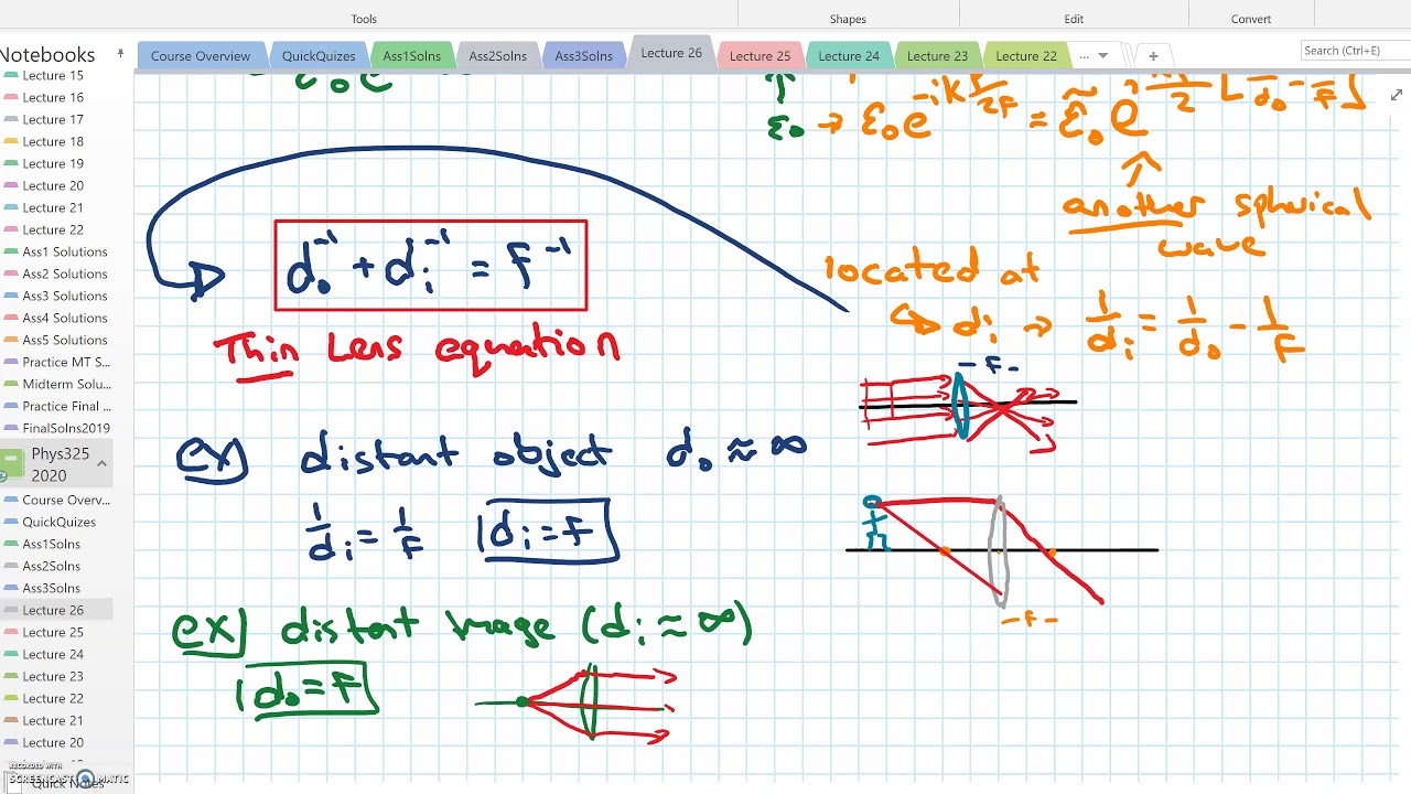
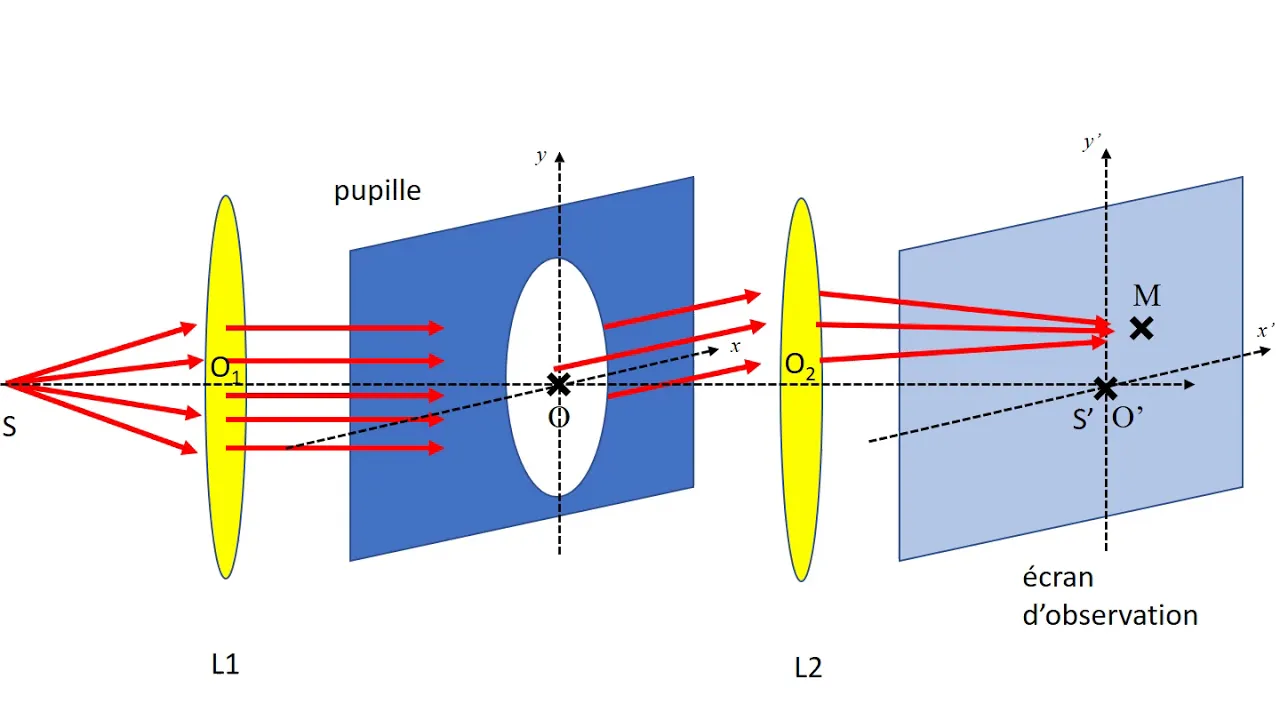
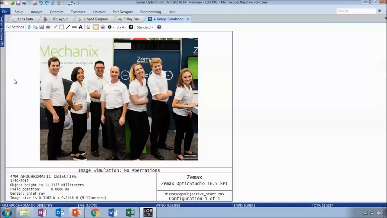
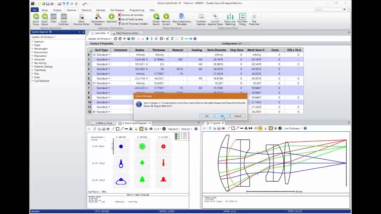
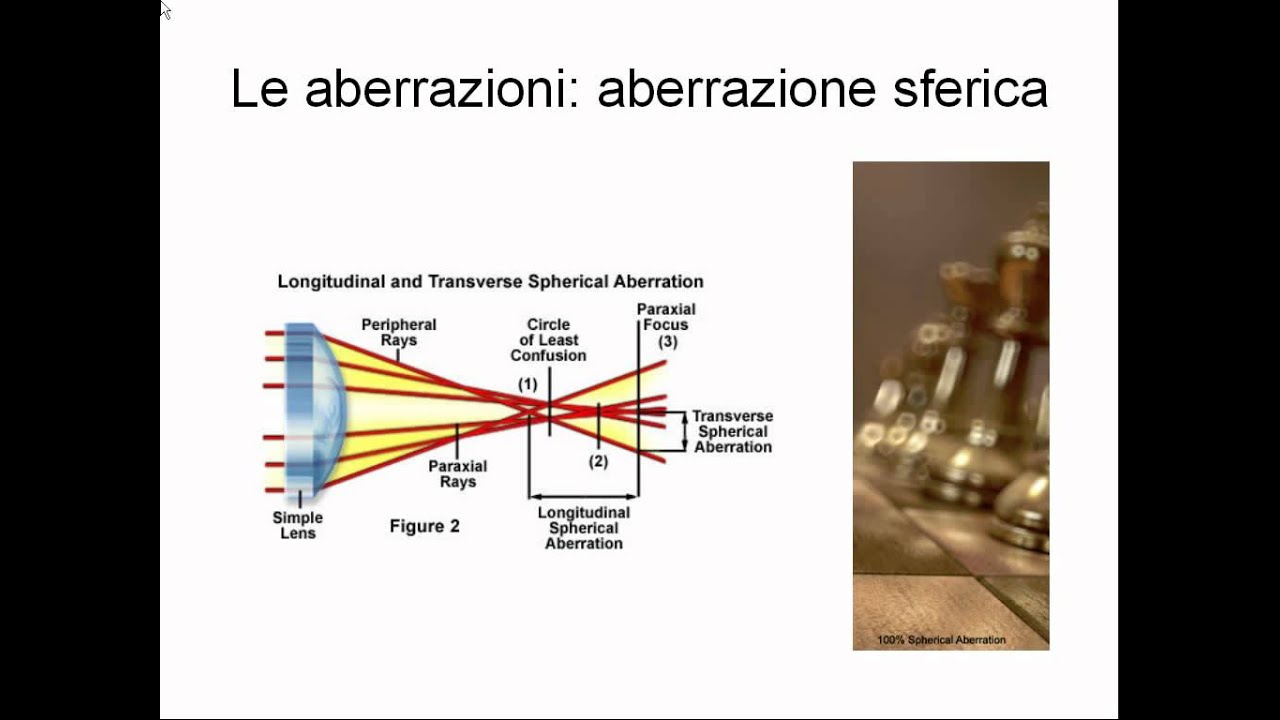
[00:00:00]we know that in an Ideal Imaging system all the light rays that come from a single object Point end up in a single image point if the Imaging system is not ideal we say that it contains aberrations in this case the light rays either don't all converge in a single point or they converge at the wrong points there may be different causes for these aberrations for example an Imaging system may be designed using paraxial Optics because then one can straightforwardly use rate transfer matrices in the paraxial approximation an Ideal Image would be formed but when the Rays make large angles with the optical axis they would not go through the ideal paraxial image point because the paraxial approximation is not valid anymore therefore the Imaging system would contain aberrations aberrations could also be a consequence of lens dispersion which means that the refractive index of the glass is different for different wavelengths the Imaging system may have been designed for a certain wavelength for which there are no aberrations but if we then use light of a different wavelength the refractive index of the glass is different and the lens elements will focus the light differently and aberrations may be introduced another possible cause of aberration is that there may be errors in the fabrication of the lens for practical reasons the lens that is manufactured will not be 100 identical to its ideal design lens elements may be misaligned with respect to each other or the shape of the lens elements May slightly deviate from the original design with aberration Theory we try to describe the way in which an Imaging system may be non-ideal in the ray model of light the physics of aberrations can be understood quite straightforwardly an Imaging system consists of a series of interfaces between media with different refractive indices the way that rays of light propagate through these interfaces is fully described by Snell's law so to see whether the light rays converge at a single image point or whether they deviate from it one simply needs to trace the race through the optical system by using Snell's law however we know that the ray model is only an approximation to the more accurate wave model of Lights it would be two computationally expensive to rigorously simulate how an optical wave function would propagate through the Imaging system so instead we would still like to use Ray tracing to simulate the Imaging system and then convert the Rays of light to an optical wave function so that we can then take into account wave effects such as diffraction describing this connection between Ray Optics and wave Optics is not entirely trivial but it's not necessarily the most difficult part of aberration Theory either the biggest part of aberration Theory consists of describing and categorizing all the different ways in which an Imaging system may be non-ideal there are infinitely many ways in which light rays can deviate from the ideal image points but when we want to understand and communicate the performance of a certain Imaging system we cannot just Trace thousands of rays through the Imaging system and leave it at that the ray Tracer output has to be processed in such a way that we can easily interpret it what helps in defining and categorizing different aberrations is the fact that there tends to be a systematic structure in the way that Imaging systems are imperfect for example if one lens element is slightly tilted it's not as if all the light rays will scatter in random directions rather there's a certain structure to how the light rays are perturbed due to a slight misalignment in the Imaging system in aberration Theory we categorize Imaging errors in such a way so that we can efficiently describe how certain imperfections in the lens system affect the image quality moreover by identifying such structures and regularities we are better able to infer system properties from aberration measurements for example if an Imaging system performs significantly worse than what is expected from the design we can describe precisely in what way the performance is worse and then we can relate this precise description to specific sorts of misalignments this helps in both evaluating and designing Imaging systems so ultimately aberration theory is not so much about fundamental physics but rather about giving names to structures so that we can talk and think about Imaging systems more easily as a result there are many different ways to represent aberrations which one needs to be aware of to avoid confusion and miscommunication in the ray model of light aberrations are described as light rays missing the ideal image points to see how aberrations are described in the wave model of light let's recall how Ray Optics and wave Optics are connected if we have array of light it propagates in a certain direction in the wave model the direction of propagation of an optical field is perpendicular to its wavefronts note that array of light can in principle be arbitrarily thin but to define a waveforms the field must have a finite spatial extent the optical field can be described as a complex valued function and the wavefronts are surfaces where the complex phase is constant if the optical field is locally approximated as a plane wave we can define a wave Vector whose Direction indicates the direction of propagation and whose length is related to the wavelength of the light this relation between Ray Optics and wave Optics explains Snell's law incident light can be described as a field whose wavefronts are separated by the wavelength of light and whose orientation determines the propagation Direction when the light goes from a medium with one refractive index to a medium with another refractive index the wavelength of the light changes at the interface the field must be continuous which means the wavefronts must still connect given that the wavelength changes this connection is only possible if the orientation of the wavefronts changes therefore the propagation direction of the light changes in such a way that follows Snell's law this demonstrates that our understanding of the connection between Ray Optics and wave Optics is indeed correct now let's see how this connection helps us describe Optical aberrations in terms of wave Optics when array of light is aberrated it means that its direction of propagation deviates from the ideal Direction since the propagation direction is directly related to the orientation of the wavefronts an error in the propagation direction is directly related to an error in the wavefronts therefore in the wave model of Optics aberrations are described as a wavefront error in an Ideal Imaging system light rays from a single object Point converge in a single image point all the Rays that converge in the image Point have different propagation directions the corresponding wavefront orientations together form a wavefront that is spherical when due to aberrations the light rays travel in different directions the wavefront orientations will change as well therefore in the presence of aberrations the wavefront will deviate from the ideal spherical wavefronts so there are different ways in which we can interpret and describe aberrations one way is to specify the mismatch between where a light Ray should intersect the image plane and where it actually intersects the image plane this is called the transverse Ray aberration another way is to specify the mismatch between where a light Ray should intersect the optical axis and where it actually intersects the optical axis this is called the longitudinal Ray aberration we can also specify the difference between the ideal spherical wavefront and the actual wavefronts which is called the wavefront error these three different ways to describe aberrations lead to different ways to visualize these aberrations to distinguish different rays of light we specify where the intersect the pupil plane to evaluate how each light Ray is aberrated we specify where they intersect the ideal image plane to create a ray fan plot we plot for a cross-section of the pupil where the Rays intersect the cross-section of the image plane alternatively we can create a spot diagram where instead of looking at a cross-section of the image plane we look at the entire two-dimensional image plane the spots that indicate where the Rays intersect the ideal image plane give an impression of the image that a single point source would creates we could also look at how far away from the image plane the Rays for different pupil points intersect the optical axis we can create a longitudinal aberration plot by plotting for each point along the optical axis from which point in the pupil the light Ray came so that it intersects the optical axis there we've now seen a few ways to visualize Ray aberrations we also stated that these Ray aberrations can be related to a wavefront error let's see how we can calculate the ray aberrations from a given wavefront error suppose we have an ideal and aberrated Ray that intersects the pupil plane at some height X and intersects the optical axis at some focal distance F away from the pupil plane the actual aberrator tray from the same point in the pupil plane intersects the optical axis somewhere else the transverse Ray aberration is given by the distance between the unaberated Ray and aberrated Ray in the ideal image plane because the two rays have different propagation directions they have different local wavefront orientations at their location in the pupil plane these wavefronts indicate where the phase of the complex valued Optical field is constant the propagation Direction which is indicated by the direction of the wave vector k is given by the gradient of the face of the wave function so if we know the phase in the pupil plane then we can calculate the propagation direction of the light Ray if we know the propagation direction of the light Ray then by using similar triangles we can calculate how much the height of the ray changes when it propagates by the focal distance f to find the transverse Ray aberration we subtract this change in height from the original height X in the pupil plane for the unaberated ray the transverse Ray aberration is zero this yields an expression for the pupil coordinate X which we substitute in the expression for the transverse Ray aberration of the aberrator trade the Z components of the wave vector k can be expressed in terms of the length of the wave vector and its X and Y components by Taylor expanding this expression for small KX and KY we find that in the paraxial approximation KZ can be well approximated as the length of the wave vector this yields a simple expression for the transverse Ray aberration in terms of the error in KX we know that KX is bound by taking the derivative of the face of the wave function with respect to the pupil coordinate X the optical path length difference or OPD is related to a phase Difference by a factor of 2 pi divided by the wavelength this Optical path length difference is used to define the way from w therefore we find that the transverse Ray aberration is given by the spatial derivative of the wavefront error from this result we can make the following important observation if the wavefront error is linear in the pupil coordinate X then the transverse Ray aberration is independent of the pupil coordinate X this means that all the Rays from different pupil coordinates still intersect at the same point so a sharp image is still formed but it is shifted laterally therefore if the wavefront error is a linear function of the pupil coordinates the image is laterally shifted but still Sharp now that we know how the transverse Ray aberrations can be calculated from the wavefront error we will now see how the longitudinal Ray aberrations can be calculated from the wavefront error by using similar triangles we can calculate at what distance the aberrated ray intersects the optical axis the longitudinal Ray aberration is given by the distance to the ideal point of intersection which is given by the focal distance f for the unaburrated ray the longitudinal Ray aberration is zero we use this expression to eliminate the focal distance f we again make the paraxial approximation where KZ is approximated as k the difference in 1 over KX can be approximated with a derivative KX can be related to the pupil coordinate X by relating the difference in KX to a difference in phase and by relating the difference in Phase to an optical path length difference we find that the longitudinal Ray aberration is given by the derivative of the waveformed error with respect to the pupil coordinate divided by the pupil coordinates from this result we can make the following important observation if the wavefront error is quadratic in the pupil coordinate X then the longitudinal Ray aberration is independent of the pupil coordinate X this means that all the Rays from different pupil coordinates still intersect at the same point so a sharp image is still formed but it is shifted longitudinally therefore if the wavefront error is a quadratic function of the Tuple coordinates the image is defocused but it can be made sharp by moving the detector along the optical axis so to summarize a linear wavefront error shifts the image laterally while a quadratic wavefront error shifts the image longitudinally so it is defocused the advantage of formulating the aberrations as a wavefront error instead of Ray deviations is that we can now use the wave model of Light which takes into account effects such as diffraction which are not taken into account in the ray model of Lights for example we saw that we can visually represent the image of a point source with a spot diagram which indicates where all the Rays from a point source intersect the image plane in the case of Ideal aberration-free Imaging all Rays intersect at a single point so the spot diagram also reduces to a single point however we know from wave Optics that the ideal image of a point source is not a single point but an Airy disk which due to diffraction has a finite extent we can calculate this Airy disk by taking the Fourier transform of the pupil to see how we calculate the point spread function or psf when aberrations are present let's recall how image formation is described in Fourier Optics in an Ideal Imaging system the field that is emitted by a point source is converted to a converging spherical wave in the fresnel approximation this spherical wavefront is approximated as a quadratic wavefront if there are aberrations present we can describe this as a wavefront error which is added to the ideal quadratic phase to calculate the field in the image plane we apply for now propagation for a propagation distance which is equal to the focal distance f this means multiplying with a quadratic phase factor and taking the Fourier transform we see that the quadratic phase Factor due to fresnel propagation cancels out with the quadratic phase Factor due to the ideal spherical wavefront in the paraxial approximation the final result is that to calculate an aberrated point spread function we take the Fourier transform of the wavefront error which is restricted to the pupil note that this formula reproduces the result we found when interpreting the formulas for transverse and longitudinal Ray aberrations if the wavefront error is quadratic it yields a phase function that has the same form as the final propagator therefore having a quadratic wavefront error is equivalent to moving the detection plane out of focus moreover multiplying a function with a linear phase shifts its Fourier transform therefore a linear wavefront error shifts the image laterally we now know how we can describe aberrations in terms of transversary aberrations longitudinal array aberrations or away front error in the following we're going to categorize and name these operations suppose we have a point source whose location is given by the coordinate Vector h this point source emits race in all directions so there are Rays going through all points of the pupil in an Ideal Imaging system all these Rays converge at a single image point the position of that image point is given by the coordinate Vector h of the original point source multiplied with the magnification of the Imaging system in an aberrated Imaging system rays that go through different points in the pupil can reach the image plane at different positions let's consider one such pupil Point whose position is given by the coordinate vector rho the light Ray that goes through that pupil Point reaches the image at the ideal image point plus the transverse Ray aberrations in the X and Y directions these transverse Ray aberrations depend on both the location of the point source and the pupil point which the light Ray that we're considering goes through we saw that these transverse Ray aberrations are directly related to the wavefront error in the pupil which therefore also depends on the location of the point source the transverse Ray aberrations are proportional to the derivative of the waveform error with respect to the pupil coordinates in the following we will assume that the Imaging system is rotationally symmetric the quantities H dot h rho dot row and H dot row are rotationally invariants therefore for a rotationally symmetric Imaging system we can express the wavefront error as a power series of these quantities the constant term in this expansion is irrelevant because the transverse Ray aberrations depend on the gradient of the wavefront error so the first terms we consider are the linear terms the first term is a quadratic wavefront error which we saw corresponds to the focus this can easily be corrected for by Shifting the image plane along the optical axis so this term is not interesting the second term is linear in the pupil coordinates and we saw that this corresponds to a lateral shift of the image of the point source we see that the image shift is directly proportional to the position of the point source which results in nothing more than the magnification of the image so this term is also not very interesting the third term does not vary as function of the pupil coordinates so it does not contribute to the transverse Ray aberrations so we see that none of the linear terms are interesting therefore we need to look at the terms that are quadratic in the rotationally invariant quantities since there are three such quantities there are six ways to pair them one of these terms does not depend on the pupil coordinates so it does not contribute to the transverse Ray aberrations we are left with five terms that describe the wavefront error as function of both the point source location and the pupil coordinates currently this function is expressed in terms of coordinate vectors but we can rewrite it as follows we Define Phi as the angle between the point source coordinate vector and the pupil Point coordinate vector this allows us to write the dot product of two vectors as a product of scalars from the expression of the wavefront error we want to find the transverse Ray aberrations which are found by taking the derivatives with respect to the Cartesian Tuple coordinates so we first need to express the wavefront error in terms of Cartesian coordinates we can straightforwardly write the radius of the Cubo coordinate Vector in terms of Cartesian coordinates by using Pythagoras's Theorem to relate the angle Phi to Cartesian coordinates we choose our coordinate system such that the point source coordinate Vector lies along the x-axis we can now Express the waveform error in terms of critesium Tuple coordinates with this expression we can straightforwardly calculate the transverse Ray aberrations by taking the derivatives to interpret these resulting Expressions we can convert them back to Polar pupil coordinates we do this by defining the relations between the Cartesian and the polar coordinates and then substituting them into the Expressions we found for the transverse Ray aberrations now we can create plots for each term to get a feeling for what they represent we call that in an Ideal aberration-free Imaging system the wavefront error is constant the transverse Ray aberrations are zero so the ray spot diagram consists of a single point however when we take the wave nature of light into account we find that the image of a point source is not a single point but due to diffraction by the pupil edges it is an airydisc this every disk is found by taking the Fourier transform of the pupil function when we look at the first term of the expression for the wavefront error we see that the error increases with the radius of the pupil coordinates we can choose a fixed radius of the pupil coordinates and then see what the transverse Ray aberrations look like we see that as we vary the polar angle Phi the transverse Ray aberrations trace a circle with a radius that scales with the third power of the pupil radius so if we consider all the pupil points that the Rays can go through we obtain a ray spot diagram that consists of concentric circles with different radii to find the corresponding point spread function we calculate the Fourier transform of the pupil function where the wavefront error defines the complex phase this aberration is called cervical aberration now let's look at the next term in the expression for the wavefront error we see that again the transverse Ray aberrations Trace out circles as we vary the polar angle of the pupil coordinates but this time these circles have an offset in the X direction that depends on the radius of the pupil coordinates the size of the circles also depend on the radius of the pupil coordinates this results in the ray spot diagram for the aberration called coma whose name has the same origin as the word comet this makes sense given their similarity and shape when we plot the point spread function we can clearly see the resemblance with the ray spot diagram we can also look at the side view of how light rays propagates when coma aberration is present we can compare the ray model to the wave model to calculate what the point spread function looks like in different planes we add quadratic wavefront errors to the coma wavefront error also here we see a clear resemblance between the ray model and the wave model next we look at the third term in the expression for the wavefront error this term depends only on the x-coordinate of the pupil and not on the y-coordinates as a result the raised Port diagram is elongated only in the X Direction but not in y the point spread function shows similar features this aberration is called astigmatism when we look at how the point spread function changes through Focus we see that first the light is focused in the X Direction so instead of a focal point we have a focal line in the y direction as the light propagates further it gets focused in the y direction so we have a focal line in the X Direction this is the key feature of astigmatism the Imaging system has different focal lengths in X and Y the fourth term in the expression for the wavefront error is quadratic which we know corresponds to the focus the thing that distinguishes this aberration from regularity focus is that the defocus strength depends on the point source location this separation is called field curvature the final term is linear in the pupil coordinates which we know corresponds to an image shift also here it's important to note that the shift depends on the location of the point source so all points of the object are imaged sharply but at the wrong location this means that the image is sharp but distorted hence this aberration is called distortion so far we've examined each term of the wavefront error in detail by looking at its race pop diagram and point spread function for a single point source however to get a clear impression of how the aberrations depend on the point source location we will have to look at an array of Point sources which all have different locations we see that spherical aberration does not depend on the point source location so all points have the same point spread function comma depends linearly on the point source location so the central point spread function is on aberrated so it's an error disk the farther away you go from the central position the more aberrated the point spread functions become depending on the sign of the aberration the coma Tails can point either inward or outward note that everything is rotationally symmetric we saw that astigmatism turns focal points into focal lines they can point radially outwards or they can point in the asimuthal direction field curvature describes how different point sources have different defocus if all points have the same defocus it means that a sharp image is formed on a flat surface when different points get different to focus it means that the surface on which a sharp image is formed becomes curved by moving a flat detector back and forth different points get in and out of focus Distortion shifts the image of different point sources by different amounts depending on the sign of the Distortion we can get either Barrel Distortion or pincushion distortion the five aberrations that we just discussed are called the sidel aberrations they are spherical aberration coma astigmatism field curvature and distortion they describe how the wavefronts error in the pupil can vary as function of the point source location they are the first five non-trivial terms of the power expansion of the wavefront error for a rotationally symmetric Imaging system related to these aberrations and coma in particular is an important Imaging condition called the Abba sine condition to understand the Abba sign condition let's first recall our understanding of what it means to create an ideal image in Ray Optics we say that to form an Ideal Image all rays that come from a single object Point must end up in a single image point in wave Optics the spherical wave that is emitted by an object Point must be converted to a spherical wave that converges in an image point but when discussing the relation between the wavefront error and Ray aberrations we saw that there is a close connection between wave Optics and Ray Optics this allows us to formulate a more stringent Imaging condition in terms of light rays that also takes the wave nature of light into account the relation between Ray Optics and wave Optics was the following wave fronts are surfaces of constant phase and phase is directly proportional to Optical path length moreover we know that the Rays propagate in a direction perpendicular to the wavefront if the wavefront is spherical and the image point lies in the center of that sphere then all the Rays that go from the wavefront to the image Point travel the same Optical path length therefore to have Ideal Imaging all the Rays that come from a single object Point must have traveled the same Optical path length when they reach the image point now let's see what this Imaging condition implies for perfectly Imaging an extended object that is if an object point B is perfectly imaged by an Imaging system what condition has to be satisfied such that a neighboring Point Q is also ideally imaged if we consider Ray Optics it is not clear how the image quality of Point Q would be affected by the image quality of some other point p but in wave Optics the two are correlated because array of light cannot be considered arbitrarily thin this is because array is assumed to propagate in a certain direction and in wave Optics the propagation direction is determined by the wavefronts which must therefore have some finite spatial extent it is this finite spatial extent that allows us to relate the image quality of one point to the image quality of some nearby point more specifically if we know the optical path length of array with a certain angle that goes from point P to its image point then we can calculate the optical path length from a nearby Point Q to its image point if Q is imaged without aberrations then the optical path lengths should be the same for all rays mathematically it means the following for aberration-free Imaging of the point Q the optical path length to its image point should be the same for all rays these Optical path lengths are related to the optical path lengths from the neighboring point B to its image point it is assumed that the image of Point p is aberration free so the optical path length is the same for all rays the difference between the optical path length between e and its image point and Q and its image Point depends on the ray angle and the distance between p and Q and the distance between their image points this difference should be the same for all Rays if the Imaging of Point Q is to be free from aberrations so the difference in path length should be equal to the same constant for all rays by considering the case where the ray is perpendicular to the displacement between p and Q we find that this constant must be equal to zero for any arbitrary array we find the optical path length Difference by multiplying the X component of the wave Vector with the displacement between p and Q which is in the X Direction rearranging this expression tells us that the ratio of the signs of the ray angles must equal the magnification of the Imaging system this is the other sign condition we can compare this condition to the condition of thin lens Imaging for thin lens Imaging the image magnification is given by the image distance divided by the object distance for a thin lens the ray must enter and exit the lens at the same height therefore we find that the image magnification must equal the ratio of the tangents of Ray angles instead of the signs of angles therefore only in the paraxial approximation where the tangent and the sine of an angle are considered equal can a thin lens create an ideal aberration-free image now let's see in what way the image is aberrated if the absign condition is violated because for example we're using a thin lens we found an expression that is proportional to the optical path length difference for different rays which is directly related to the wavefront error this expression can be written in terms of the signs of the ray angles using the expression for image magnification and the tangent condition for thin lens Imaging we can rewrite the expression for the optical path length difference to see how this difference changes as function of Ray angle we note that the difference between the sign and tangent of an angle scales with the third power of the angle therefore the optical path length difference goes linearly with point source location and with the third power of Ray angle noting that the ray angle directly determines where the ray goes through the pupil we find that this expression for optical path length difference corresponds to the coma aberration so we found that a single thin lens cannot satisfy the ab assign condition and that violation or offense of this condition leads to coma a lens that satisfies the absign condition and has no on-axis aberrations is therefore free from spherical aberration and coma such a lens is called an aplanatic lens we can interpret the absoline condition in a different way by using Fourier Optics array with a certain direction of propagation corresponds to a certain point in Fourier space which is the pupil the sine condition states that all these points are scaled by the same factor therefore the Imaging system simply scales the Fourier transform of the object which leads to a magnification in the image however if the sign condition is violated the points in Fourier space are not scaled linearly which means the pupil gets distorted and the image gets aberrated therefore violation of the sign condition is typically associated with coma as well as pupil distortion the sidel coefficients are one way to describe the aberrations of a rotationally symmetric Imaging system another way to describe aberrations is to use cernica coefficients away front error in the pupil can be written as a linear combination of cernica polynomials where the weights are discernica coefficients of course you can always write one function as a linear combination of other functions so what's special about the zernica polynomials one thing is that they form an orthogonal basis on the unit disk that is any arbitrary function can be written as a linear combination of the cernica polynomials and the coefficients can be straightforwardly found by taking the dot product of the function with the zernica polynomials secondly the lower order polynomials can be straightforwardly related to The Familiar aberrations such as coma and astigmatism let's look at the definition of the cernica polynomials they are defined by two indices the two indices n and M together Define the radial dependence of the function while only the second index M defines the angular dependence for the first polynomial both indices are zero the function is constant and it is called piston for the next two polynomials the first index n is one the second index M ranges from minus n to n in steps of two so here n can be equal to -1 or 1. note that as we vary the angle the function undergoes one period because the index M has a magnitude of one the aberrations are called tilt and since they describe a linear wavefront error they cause a shift in the image for the next set of polynomials the functions undergo either two periods when we vary the angle or their constant the defocus aberration is quadratic so the image is shifted along the optical axis the other aberrations correspond to two orientations of astigmatism in the next set of polynomials we find the comma aberration in different orientations these are the first several cernica polynomials in an infinitely long list when we describe wavefront errors in terms of zernikes it is important to be aware of the different conventions that can be used we saw that the cernica polynomials are defined with two indices n and M however we often want to list the polynomials with just a single index and there are several conventions on how to convert the two indices to just one moreover there are different conventions on whether the polynomials should be normalized therefore if we Define a set of zernica coefficients to describe a wavefront error it is important to be clear with which conventions these coefficients are defined now let's have a look at the differences between describing wavefront errors with sidel aberrations and with cernica polynomials when we Define facidal aberrations we used an expression for the wavefront error that depends on both the pupil coordinates as well as the point source location as a result we could create a picture that shows how Point sources at different locations yield different point spread functions the cernica polynomials on the other hand depend only on the pupil coordinates that is they can be used to describe a wavefront error but not how that wavefront error depends on the location of the point source if we want to specify this dependence we would have to Define for each point source location a separate set of cernica coefficients however the limitation of the sidel aberrations is that they assume that the Imaging system is rotationally symmetric the zernica decomposition does not need to make such an assumption there are also some subtle but important differences in how certain aberrations are defined for example when we compare seidel's definition for spherical aberration to zernica's definition we see that zernica's definition has an extra defocus term this is necessary to ensure that the different surgical polynomials are orthogonal seidel's definition of coma is the same as zernicus except for an extra linear term which corresponds to tilts the definitions for astigmatism differ by a defocused term recall that if an Imaging system has a stigmatism it has different focal lengths in the X Direction and Y Direction so there are two different planes where there's a focal line in the X Direction and in the y direction indeed if we add to the cernica polynomial for astigmatism a defocus term we find that the light is focused in One Direction and if we subtract the defocus term we find that the light is focused in the orthogonal direction therefore the zernica polynomial for astigmatism describes what the wavefront error is for the field exactly between those two focal lines field curvature is described by the cernica polynomial for the focus and Distortion is described by discernica polynomial for tilts the key point is that the coefficients for these cernica polynomials would have to depend on the point source location to actually describe field curvature and distortion we can also look at the point spread functions of the sidel aberrations and their corresponding zernica polynomials horse spherical aberration the effect of the extra defocus term in the zernica polynomial is clearly visible in the point spread function for coma the wavefront errors look quite different but the only difference in the point spread function is that it is shifted rotating the wavefront error will also rotate the point spread function the zernica polynomial for astigmatism yields a point spread function with the shape of a cross this confirms that the polynomial describes the field exactly in between the horizontal and vertical focal lines that are typical of astigmatism also here we have a rotated cernica polynomial which has a rotated point spread function now let's imagine how these Concepts would be used in practice suppose we have designed some Imaging system that consists of a series of lens elements placed at specific positions if we could manufacture the system exactly as designed its performance would in some sense be ideal or nominal however due to practical reasons there will always be some errors in the fabrication lens elements can be slightly misaligned in different ways if a lens element is displaced along the optical axis it's called d space if it's displaced perpendicular to the optical axis it's called the center and finally a lens element can be tilted the more accurately we want to align the system the more expensive it becomes therefore to produce Optical systems in a cost-effective manner it is important to specify whatever it is allowed to have one way to quantify the error is by using the magnitude of the wavefront error one can use Ray tracing software to see how misalignments of different lens elements affect the wavefront error the wavefront error may be very sensitive to the misalignment of one lens element but not another so some lens elements would have tighter tolerances than others moreover different sorts of misalignment will affect different types of aberrations for example if a lens element is despaced the optical system is still rotationally symmetric therefore these spacing will affect the presence of rotationally symmetric or cervical zernicus but not the other cernicus at least on axis on the other hand if a lens element is tilted or decentered asymmetric cernicus such as on-axis astigmatism and coma will be affected once an optical system has been manufactured its wavefront error can be measured experimentally this wavefront error can be decomposed in cernicus and the resulting coefficients can then be communicated and interpreted so if we were presented with a set of coefficients what can we learn from them first note that sometimes the first few coefficients are not given this is because they correspond to piston tilt and defocus they are not very interesting because piston does not affect the image tilt only shifts the image laterally and the focus can be corrected for by moving the detector along the optical axis so how do we interpret the remaining coefficients first we need to interpret the indices correctly as we saw a moment ago there are many different conventions to turn the two indices of cernica polynomials into a single one so we first have to know which convention is being used here let's say the so-called Fringe indexing was used in this indexing the indices which are squared numbers correspond to the rotationally symmetric zernikes since we see the coefficient Spike at indices 9 and 16 which are squares it seems that in this Imaging system the aberrations are rotationally symmetric these aberrations may be part of the nominal design in which case there is no problem but if the values are unexpectedly large there must be some error in the system that causes these aberrations while still retaining rotational symmetry for example one of the lens elements could be the spaced but it could also be that one of the surfaces has the wrong curvature or perhaps some of the materials in the Imaging system have a different refractive index than expected in any case these cernica coefficients tell you something about the image quality you can expect from the system and they can give Clues to what may have gone wrong in the manufacturing if anything