






















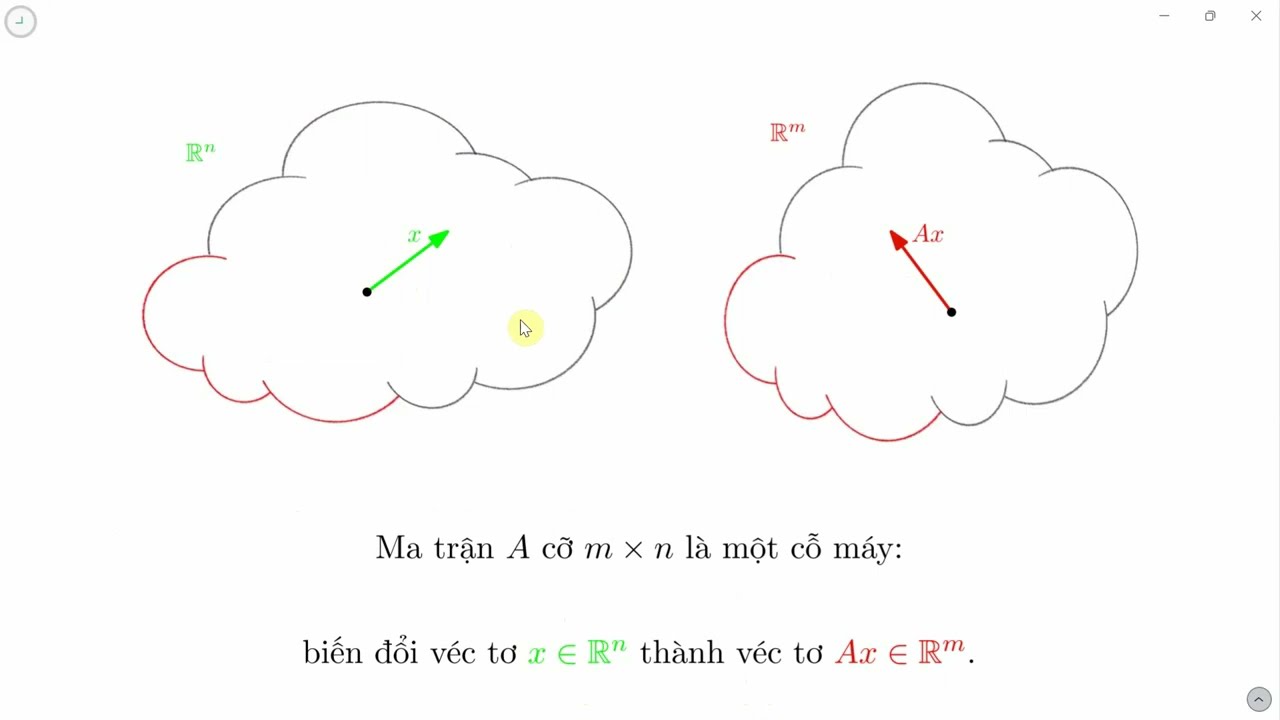
![[Linear Algebra] Geometric Transformations](https://i.ytimg.com/vi_webp/7Hj9AnBTfTE/maxresdefault.webp)
![[이얼 전공수학] Lay 선형대수학 제12강 -1.9절 선형변환과 행렬(1)-](https://i.ytimg.com/vi/mQ11DuYgd7Y/maxresdefault.jpg)


![[핵심 머신러닝] Principal Component Analysis (PCA, 주성분 분석)](https://i.ytimg.com/vi_webp/FhQm2Tc8Kic/maxresdefault.webp)


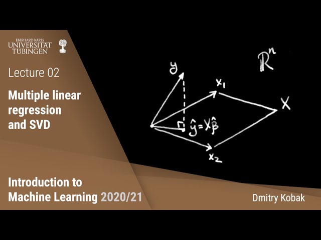


In machine learning, matrix-vector multiplication (XW) computes predictions for all training samples simultaneously by performing inner products between each row of the feature matrix X and the weight vector W, where the number of columns in X must equal the number of entries in W for the operation to be valid. This operation enables compact representation of linear models, and matrix factorization (X = UV) allows decomposition of data into latent factors, with the minimum number of factors (R) corresponding to the matrix rank, which represents the minimum number of outer products needed to reconstruct the original matrix.
Vectors, Matrices & Matrix Multiplication | ML Foundations (UChicago) | Lecture 2
Added:Basic algebraic operations, including working with variables, linear equations, and Cartesian coordinate systems.
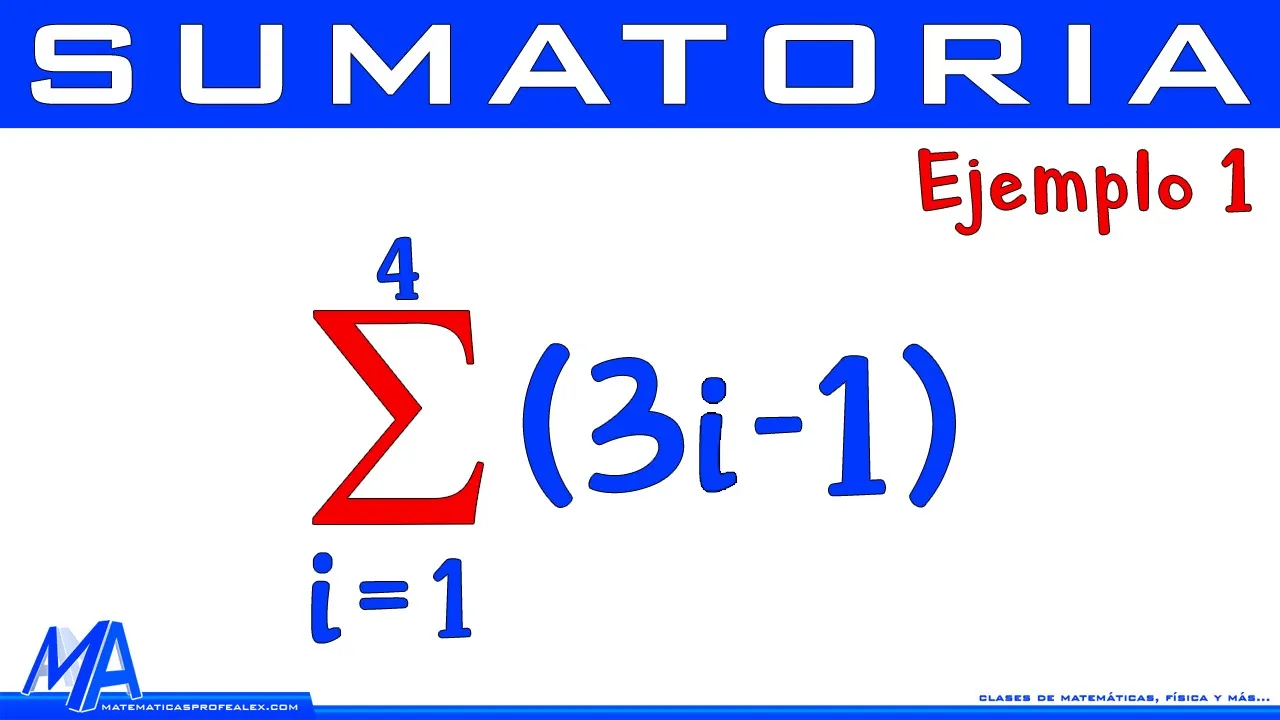
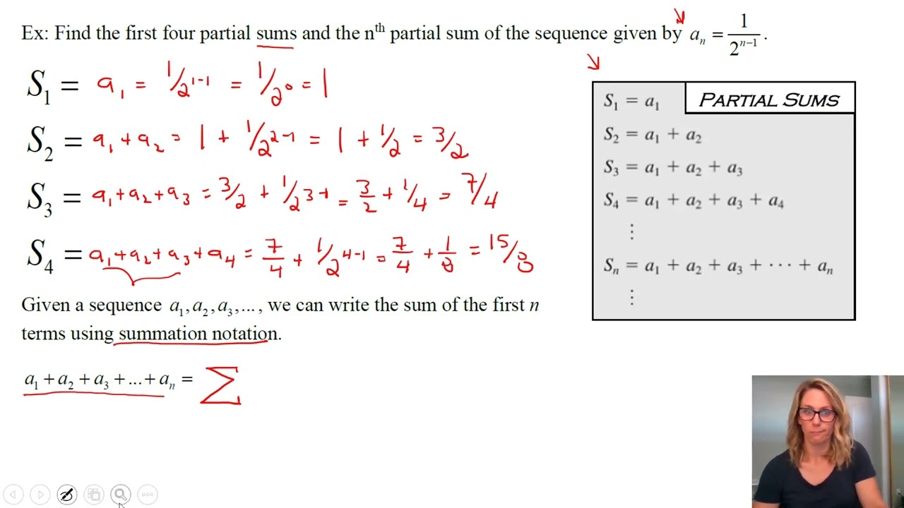
The concept of summation notation (sigma notation) for representing the sum of a sequence of numbers.
Fundamental geometric concepts such as distance, length, and the Pythagorean theorem in multi-dimensional space.
Familiarity with basic data representations, such as tables of data, arrays, or lists, to understand how data translates to vectors.
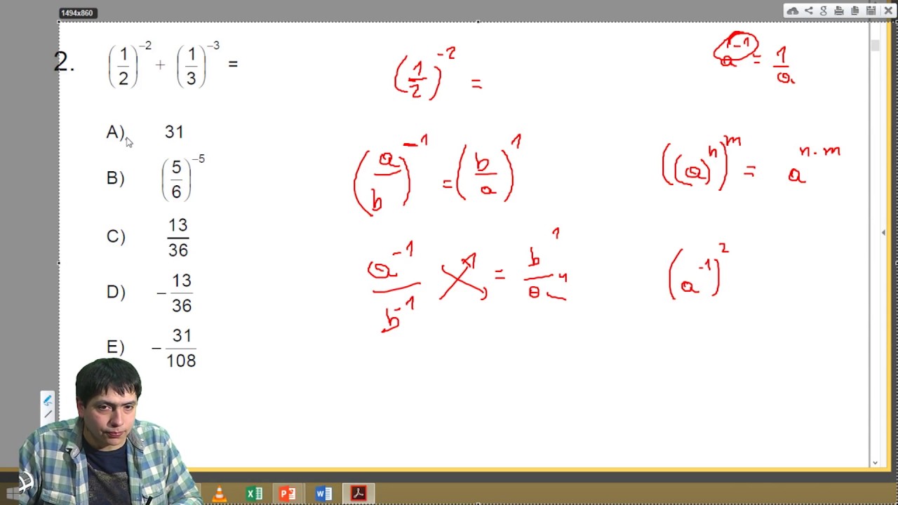
Matrix properties and operations such as transposes, determinants, and matrix inversion.
Systems of linear equations, understanding vector spaces, span, linear independence, and basis.
The geometric interpretation of matrix transformations, including scaling, rotation, and projection.
Eigenvalues and eigenvectors, which form the mathematical foundation for Principal Component Analysis (PCA).
Applying vector and matrix notation to formulate and solve linear regression models (least squares) models in machine learning.
794 views17likes1:15:23Original Release: 2025-10-03
All right, welcome back everybody. Um, a quick note on logistics. Uh, my office hours can be hard to find. So, they are in this building on the first floor in the annex. So, you know, the main entrance that's down below there. If you were to come in that way, you would just keep on going straight past the main hallway, past the bathrooms, past this little hallway that has another entrance, and then you that's the annex.
And as soon as you're in the annex, it's immediately to the right. It's N175.
So, um hopefully that helps. But, um office hours will be um are posted on the uh on Canvas site, but just in case you have trouble finding the room, I wanted to make sure everybody knew. All right. So, today um we are going to start uh by talking about matrices and vectors.
[Music] And if you recall from last time, we started off by saying that we had training data that we wrote as pairs of feature vectors x i and labels y i for i= 1 2 n.
Um, and to start off, we're thinking about classification.
So the yi would be a label say +1 or minus1 and x i this vector of features we write as x i1 x i2 all the way to x i p for our p different features. And we say this is in RP with this fancy bold R here to indicate that there are P different entries and each one is a real number.
Um and so XIP is the P feature of the E sample. Um and so then we said we wanted to consider a linear classifier [Music] and in particular we wanted our predict to predict um a label Y hat for a sample or a feature vector.
[Music] X knot. And if you recall, I'm using Xnot to correspond to just a generic feature vector um when we're training.
It could be one of the training feature vectors, or this could be a new sample that we want to make a prediction on that's not in our training set. And the way we do this with our linear setting is we're going to say xhat is going to be a weighted sum of our features. So we're going to have weight 1 * x i1 plus weight 2 * x i2 all the way to weight p * x.
So what we said before is that we could also have a weight vector [Music] W and that just has all of our different weights in it. W1, W2, all the way to WP.
And so this is also in RP because it is a vector of real numbers and there are P different entries in it.
So now that we've got these vectors of the feature vector and the weight vector, we can establish basically some shorthand for writing these weighted sums that we're going to be dealing with. And so last time we said there were four different ways we could write this. We could use these angle brackets and write this as w and x knot inside the angle bracket. Um the order doesn't matter. So we could also write it as x knot and w in our product. And we said we could also write this as w transpose * x knot. And we could also write it as x knot transpose * w.
All of these are equivalent um ways of writing this weighted sum and we call it an inner product.
[Music] So in this setting now we are going to predict new labels for a new feature vector by taking the inner product of that feature vector with a weight vector. And what we're building towards is of course figuring out what is a good weight vector to use based on all of the training samples that we have.
Are there any questions so far?
Okay, so so far we've been forming vectors for each individual training sample and for the weight vector, but we're going to form additional vectors correspond that go across all of our different samples as well. So we can also form a label vector.
So this is y underline and this just has the labels y1 y 2 all the way to yn. So this is a vector in most generally um it's in Rn like when we start talking about regression or settings where the y's could be any real numbers but for classification um we would have it be in + one or minus one um again to this p uh n power. So this is telling us that our vector has n different entries and each entry is either a plus or minus one in this case.
Finally, we can form a feature matrix.
And basically, all we're going to do is take all of the feature vectors for all of the training samples and put them together in one big construct.
Okay, so this is going to be like a whole bunch of vectors concatenated together. So it's going to be a matrix in R N by P. So this is telling us that the entries are real numbers. There are n rows and there are P columns.
And so what we're going to have here in the first row is the feature vector X1 corresponding to the first training sample. Now, if you remember when I wrote each of the x's before, it was a column vector. So, but now I'm telling you I want this to be a row. So, I'm going to write transpose here. So recall that when we talk about um the transpose [Music] if we have a vector x let's say um x knot and we transpose it then this is just x1 x2 all the way to xnot p like that.
Okay, so it's the same information, but we're now representing it as a row instead of a column. And so in our feature matrix, our first training feature vector X1, we transpose it, makes it a row, and then that becomes the first row of the matrix. And then we're going to do the same thing with X2, and that becomes the second row. And we go all the way down to XN for our N different training features.
Any questions about this so far?
>> Yeah.
[Music] are we not intended to use the X?
>> Oh, you know what? Thank you very much.
Um, I did mean to write XO here. So, thank you. I mean, I guess in general, right, we're just taking the entries of a vector that we want to make a prediction of. So, this is Y hat that's being predicted on for XO. So now if I wanted to make a predicted label for an x i then I would replace this with x i.
So it's just a generic formula but thank you very much. Yeah that's exactly right.
Okay so in this matrix when we talk about x i j oh so first of all I'm going to call this c matrix capital x. I'll try to be clear about capital versus lowercase X's on the blackboard but if if it gets confusing let me know. So in here xigj is equal to the i row j column and also just like we talked about last time it is equal to the j feature of the i sample.
So the E row of X of the big matrix X is going to be equal to the P features of the E sample.
Um and more generally like in in this particular case um we are writing this as x i transpose like I said over there but for a generic matrix that doesn't necessar if we wanted to talk about the e row of that matrix we're going to use the notation capital x i comma dot So this is indicating we're taking the e row and then we're taking all the entries in that row. And this is the notation used by the textbook that we're using for the class. Yes.
>> So if x is a sample, why are we calling there like a feature instead of a sample?
>> So the whole point of the the question was why if x is a feature are we using x knot instead of like the training features?
>> Like if x represents a sample and the sample has multiple features why we are saying we predict yhat for a feature instead of for samples.
So when I talk about samples versus features I think of each one of these pairs x i yi as being one training sample and then I say for that training sample I have p different features of that sample. So we talked last time about this um problem of taking a image and to determining whether the face was smiling or not. So the X eyes would be different distances say on the face between the eye and the mouth for instance. So each sample would correspond to a different photograph with its own label and then for that photograph we've got multiple different features.
Does that answer your question? Or maybe I misunderstood.
>> No, I think there is like kind of a typo.
>> Okay.
>> What's the typo?
>> Oh. Oh, for a feature vector. Sorry. Is this what you mean?
[Music] >> Is that what you're getting at?
>> Okay, great.
All right. Any other questions?
Okay. Um and then finally we could have the I'll just start in the new board. Um the J column of this matrix X and when we talk about the column it means the in this context value of the J feature across all the training samples.
and we are going to write it as x dot comma j. So this means we're selecting the j row um j column and we're are taking all of the entries across all of the rows for that column. And again this is the notation used by your book. So um hopefully that'll get reinforced.
So now with this we can write our linear model [Music] as the following. So y hat now with the underline is going to be all of the predictions for all of our training samples.
So this is going to be y hat i or I'm sorry y hat 1 y 2 all the way to y hat n. And if we find a good learned model then the y uh label vector for our training data and this predicted vector are going to be the same or very close to one another. But in general, they're not the same thing. One is coming from whoever labeled our data and the other is the output of our model. Now, we can write this as the product of this matrix X with our weight vector W. And so now we're going to do is learn about taking the product between a matrix and a vector. But hopefully you can start to see how this is giving us a little bit of helpful shortorthhand because when we started off we had to start with a single feature vector and then we could make a single prediction. And now we have this handy way of compactly writing all of our training data and all of our predicted outputs for all of our samples in one compact formula. And this is going to allow us to do a lot of algorithm development and thinking about how different methods work um much more easily than if we were writing out these long weighted sum equations everywhere.
Okay, so next we want to look at the matrix vector product.
[Music] So like for instance x * w.
So what this means is that if we were to look at the in the i entry of y hat. So the i entry of the result of doing this product.
Then this is equal to the inner product of the E row of X and this weight vector W.
So when we write this matrix vector multiplication, all we're doing is n different inner products exactly like we wrote on the first board. I'm just doing them one after another and then stacking them on top of each other. So if you recall the i row of x was equal to this i feature vector x i and then we take the inner product of that with w.
So we can write then um this product y hat which is the product of x and w um as being equal to this vector where the first row is the inner product of x1 and w and the second entry is x2 inner product with w all the way to the nth entry where we have x n inner product with w.
So it's just a collection of inner products.
And so again, we've got this like very simple, neat, compact formula that's representing weighted sums for all of our different training samples um in a very simple and easy to read way. Yes.
Why is it in here we do notate x i xpose?
>> When we use this angle notation then we don't use the transposes. But this is equivalent to saying x1 transpose * w x2pose * w all the way to xnpose * w.
Exactly the same thing. Great question.
Any other questions?
[Music] So, one thing that I find to be really helpful to keep in mind is this notion that dimensions [Music] must always match.
It's a really simple concept, but every time I have a bug in my code, it's the first thing I check. So, it's just helpful to make it explicit. So, in particular, we have this expression yhat is equal to xw.
And so, I picture this as follows. I've got my vector of predicted labels y hat and the number of entries in this was n and this is the product of a matrix x and I just want to make this a little bit more extreme actually so it's clear that n and p are different. So this is x which has n rows and p columns. So this is n and this is p and then we multiply that by w vector which has height p and this was yhat.
So for the matrix vector multiplication to work the number of columns in x has to equal the number of entries in w because we're always doing inner products of each row with w. So in order to do the weighted sum, they have to have the same number of entries. And then the product is going to have the same number of entries as the number of rows in X. Okay, I maybe this sounds kind of obvious, but again, it's a very, you know, if you're just coding and for instance, you're getting some error about um not being able to multiply two things, the first thing to always check is whether you've got your dimensions right or whether you've accidentally like taken the transpose of something.
Okay, so um let's see.
I also want to revisit this notion of transpose because I talked about it for a vector. But we can also transpose a matrix. So if X were equal to the 1 2 3 4 5 6. So if this were our matrix X then taking the transpose of it X transpose is 1 2 3 4 5 6. So we're just sort of like pivoting it. You can imagine there being like this diagonal that we're pivoting around so that each row becomes a column in the transpose matrix.
Okay. simple concept, but it'll be um uh uh useful later. And in the lecture notes that I'm going to post online later today, there's a link to a Wikipedia file that has a really nice graphical illustration of this that I think might be useful.
Okay, I also want to just mention a couple of basic facts that I think will be useful. Um, [Music] so imagine that we've got two vectors A, which is A1 through A P and B, which is B1 through BP.
Then if we were to write a + b, that just means that we add up each of the entries. So a1 + b1 all the way to a p + b p.
And if we were to talk about the norm of a vector and specifically I mean the uklidian norm.
We would write that for this vector a say using these double lines on either side and implicitly we typically mean that there's a little two there and we'll talk more about alternatives to this later on and what would mean if we didn't have a two here but for the most part when you see these double lines without any number underneath it means the definition that I'm going to give view which is simply that we take the inner product of a with itself and then we compute the square root of that. And the intuition here is that if we were to think about this in 2D space which is really the easiest space to draw in. Then if we were to say, so if one axis was the A1 axis and the other axis is the A2 axis and we plot our vector A right here, then this uklidian norm is basically telling us the distance between that point and the origin.
Okay, so there's a nice geometric meaning. Um and then finally we have the outer product and we'll talk about outer products. Um well I'll just say it right now. So before when we had an inner product we would have a transpose b. For the outer product we're going to have a b transpose.
So remember a now is in this case p by 1 and b transpose is 1 by p. And so what happens when we multiply these together is first of all we always have this sort of dimensionality. So what happens when we multiply these together is that the inner dimensions are going to cancel out and the result is going to be a p matrix. And what's in that P by P matrix? Basically, we're going to have A1 B1 A1 B2 all the way to A1 B P and then we have so basically we've got A1 the first entry of A times the entire vector B transpose and that gives us our first row. And then we have a2 times the entire vector brpose. So a2 b2 a2 b1 a2 b2 a 2 b p all the way down to a p b1 a p b2 to a p bp.
[Music] Okay. So basically what this is giving us is um like I said a1 * the vector brpose a2 * the vector brpose all the way down to a p * the vector brpose.
Okay so simple concept but the basic thing to remember is I can take these two vectors and compute this outer product in order to form a full matrix and this is something that we will see in a little bit. Are there any questions?
Okay. If not, then I want to work out um a small example that's tied to um our machine learning setting.
[Music] So in particular, let's say that our feature matrix X has entries 1 2 0 0 0 3. So our first training sample has features 1 0. Our next training sample has features two 0. And our final training sample has features 0 and three. And so in this case n the number of training samples is equal to three.
and P the number of features is equal to two.
And so X1 our first I said this verbally but I'll just be explicit here. X1 is 1 0 X2 is 2 0 and X3 is 0 3. So we can extract that exactly from this feature matrix.
Now if the weight vector W had entries two and four then we can ask what would be the predicted weights I'm sorry predicted labels associated with these features and these weights and to get that we are going to do matrix vector multiplication [Music] So in particular if we wanted to compute um yhat vector which is x w then the first entry of this is going to be the inner product of our first feature vector x1 and our weight vector w. And then we're going to do the same with feature two. And then we will do the same with feature three.
Okay. So for the first entry, we're taking the inner product of this weight vector with this feature vector, which is just the weighted sums of the entries. And what do we get?
>> Two. And what do we get when we do the inner product of the second feature vector with W?
Four. And what about the final one?
Sorry, >> 12. Yes. Excellent. Okay.
Very nice. Now, this is one way that we can represent this matrix vector multiplication. Alternatively, we can say that this is equal to what what we're doing here is computed a computing a weighted sum of the columns of x.
So in particular, I've got my first column of x, which is 1 2 0. And I'm going to multiply that column by my first weight, which is two. And then I've got my second column 003.
And I'm going to multiply that times my second weight, which is four. And so when I'm multiplying a vector times a scaler, just multiply that scaler times each entry in the vector. So I get 2 4 and 0. And then I get 0 0 and 12. And when I add these together, I get 2 4 and 12. So both totally valid ways to think about this matrix vector multiplication.
And depending on the context, one can be easier than the other or or more helpful than the other. So this is really nice because there's this very clear and direct link to this notion of weighted sums of features that can feel very intuitive. And when we start talking about le squares next week, what we're going to see is that this notion is going to connect directly to notions of spans of subspaces and a geometric interpretation of le squares. So both are extremely helpful.
[Music] Okay, any other questions?
All right. Now, we've been talking about linear classifiers or fitting lines to data um or doing things with weighted sums.
And this might feel a little bit restrictive to you, right? How often does your data really line up nicely with a straight line? And so I want to go through another example that highlights [Music] how with some simple manipulations we can do something much more powerful with a simple linear model. So in particular let's imagine that we observe um our data like this. And so the obs I'm going to use the letter Z to correspond to an observed feature.
And I'm going to say how this is connected to the features X that we've been talking about so far in just a minute. But just think about this as more like the raw data features that we observe. And then on the vertical axis we'll have the true labels Y.
And then imagine that when we do a scatter plot of our data, we see something like this.
So at first we might feel a little discouraged because if we were to say, "Oh, I want to try to fit a line to this data. I know right off the bat it's not going to be very good." But it turns out that the simple linear model that we've been working with can be used to fit curves like this with relatively little effort. And so that's what we're going to work out in this example.
[Music] [Music] Okay. So in particular, what we could do is we could define our feature vector XI to not just be the observed feature Z, but to be something more complex. So in particular, I'm going to have the first entry be one, the next one be zi, the next one be zi squared, and the last one be zi cubed.
So I'm taking a single measurement zi and I'm transforming it into a vector by looking at different powers of that zi. And so now we've got a feature vector.
And so now if I were to use a linear model, well, first of all, this is going to give us a feature matrix X that will look like 1 Z1 Z1 2 Z3 squared all the way down to 1 ZN ZN 2 ZN oops cubed. Sorry.
Like that. Okay. So, I have um put all of my feature vectors into my feature matrix. Um and so now if I were to think about what my linear model is doing. So, y hat for the i sample is going to be a weighted sum of these different features in my feature vector. So, I'm going to have weight 1 * 1 + weight 2 * z i + w3 * z i^ 2 + w4 * z i cubed.
[Music] And so now what we see is that the linear model on the uh features on the x's is the same thing as a polomial model on the z's.
and the weights in the linear model are the same thing as our polomial coefficients.
So again we're focusing on linear models here but it's an extremely powerful tool that can do things many things including fitting nice polomial fits to to data.
Okay any questions?
Yeah >> I guess now we can a scaler as our feature but um that's kind of sacrificing capability of the linear model to handle high dimensional data. So is there a way to both the nonlinearity and the multivariables?
>> Okay. So if I understand correctly, the question is what if I were to observe instead of a single zi say uh for each sample maybe the observed features are say two-dimensional a three-dimensional what can I do? So if I were to have each zi be a vector that let's just try to keep the writing minimal that has entries zi1 and zi2 then I can still play a very similar trick where I could form a feature vector x i that maybe is one zi1 zi2 zi1 squared zi2 2^ 2 oops okay zi1 zi2 etc right so I can still form polomials of multiple variables to get these higher dimensional features um explicitly later in the quarter we'll talk about things like kernel methods that do this implicitly and give us a major boost in performance in a lot of different settings but we're going to hold off on that for a few weeks. Any other questions?
All right. So, what we've been doing so far is talking about products between matrices and vectors, which are important.
But now we're going to move on to talking about products of matrices with matrices.
[Music] Okay.
[Music] Now, you can find any number of sources on the internet that will show you like the recipe for computing matrix matrix products. It's not hard. It's just a whole bunch of inner products. Um, but I want to give you a little bit of intuition about what's happening with these products and how it relates to machine learning. And so with that in mind, I want to think about a motivating example related to recommener systems.
[Music] And I mentioned this briefly when we when we were going through the initial slides on Tuesday, but imagine for instance that you very luckily ran Netflix and you've got a database of customers. So maybe Becca and Tion and Victor and Michael. And then I'll just I don't want this to be opaque later.
[Music] And then you also have a library of different movies. So you've got Star Wars, Pride and Prejudice.
Uh what did I put? Barbie, and Halloween.
And then for each person, let's imagine that we know how much they liked each of those movies. Um, so I'm going to use the numbers in my notes so that we can do uh some concrete examples later on.
So I've got 6 475 48 26.
Ah.
[Music] [Music] Okay. So, this is our matrix of ratings.
Now, of course, in real life, we wouldn't know how much everybody likes every movie. We would only observe a subset of these entries, and we would then try to fill in the missing entries.
And we are going to talk about exactly how to do that later. But in order to do that, we have to know how to multiply matrices matrices with each other. And so, for the moment, just to understand a little bit about matrix matrix products, let's assume we've got this entire matrix.
And what we're going to do is we are going to write it as the product of two matrices.
[Music] So I'm calling this matrix here capital X. So we're going to write X as the product of two matrices [Music] U and V.
And in this I'm going to have x be like we've been doing so far [Music] n by p. So I've got n different rows and I've got p different columns. And I'm going to write this as the product of a matrix u that in this case has n rows.
I've got to have the same number of rows as X, but only R different columns.
And a matrix V that has R rows and P columns.
So this is still R and this now is P. So I've set this up in a way so that when I multiply these together again we can always check dimensions and what's happening is when I'm multiplying these together all the r dimensions they're basically going to be inner producted together and so what I'm going to be left with is a product where the number of rows is the number of rows in U and the number of columns is the number of columns in V. And in order for this to work out, I need the number of columns in U and the number of rows in V to match up. So I can do a whole series of inner products that I'm going to describe. Now, are there any questions?
[Music] Oh yeah.
>> So here we're [Music] like to be like like why is >> I don't have any transposes here. We could write we could represent matrices in ter in terms of transposes but I think that's not the easiest way to introduce the notion of matrix matrix multiplication. So what I'm saying here is simply that x is equal to the product of u and v and I'm going to describe what that means in more detail.
Yeah.
Okay. Um so in the context of our example we could um think of for instance u um let's say the r columns of you being equal to the tastes profiles of our representative movie watchers.
Um, and so this could tell us, for instance, the first column of U could tell us how much a romance lover would like each of our movies, and the second column of U could tell us how much a horror lover likes each one of our movies. And then we could think about uh V.
So the P columns of V tell us how much each of uh the P customers resemble um the R representatives.
So, if I'm one of the customers here, sorry, I have to step on the thing to make the camera move. Um, if I'm one of the customers here, then there's R numbers in here and they're telling me how much I'm The first one would tell me how much I'm similar to the first column of you, say the romance lover. And the second number would tell me how much I'm similar to the second column of you, say the horror lover. Right? So the V is now telling me for each of our P customers, these R numbers tell us how similar we are to each of the R representative columns in U.
And so in terms of the mechanics, um I know we're just about at time, but I just want to not start this completely over when we resume on Tuesday. If x is equal to uv, what that means is that if I were to look at the i j entry of x and remember this means i row j column. If I were to look at that entry of X, then this is going to be the inner product of the I row of U with the J column of V.
So I can write this pictorially now. Um, yeah, I'm just going to redraw it. So if I've got my matrix X here and it is the product of U and V.
And now what I want to do is I want to know if I were to choose the E column of X and the I'm and sorry the E row of X and the J column of X. So if I wanted to know that entry there, then what I'm doing is I am looking at the E row of U which has R entries and the J column of V which has R entries and I'm computing their inner product with each other. And so as I go through this matrix and I look at different entries, say as I go through different entries in um one row of X, I'm just computing the inner product of the E row of U with different columns of J. And as I were if I were to compute different elements along this column in X, then I'm continuing to hold this column of V fixed and I'm just varying which inner product or which row of U I'm computing an inner product with. So this notion of inner products that we started off the day with that was it central to this notion of linear models is also central to the notion of how we compute products of matrices with vectors and also central to the notion of how we compute products of matrices with themselves. And next time we'll see just a little bit more um on this but please do read the notes. I think there's a little additional nuance on notation or things are explained more than once in a way that might be helpful. So, don't hesitate to look at the written notes and um ask any questions you might have.
[Music] Thank you very much. Okay, so what is a column [Music] of X? Um so we're going to write that as x uh dot comma j like I mentioned before. So this is the J column of X and the size of it now is going to be um uh sorry well if X is a matrix in R N by P then the J column is going to be a vector that is um length N.
And we can also think about this as a weighted sum of the columns of U where the J column of V tells us what the weights are.
So this is the same as taking the full matrix V and computing the product of that matrix with the J column of V which we write as J do I mean V dot comma J.
Um and in the context of our running example, this is the expected tastes of our J customer.
[Music] And similarly we can think about a row of X in terms of this matrix matrix product. And think about what that means.
[Music] So in particular we write that row X I comma dot. So e row and then all the entries in that row. So this is the i row of x and this is a vector that has p entries but I'm going to write this as r one by p to indicate there's only one row and p entries across that row.
And we can also write this as taking that matrix V and computing the product of that matrix V with the U I'm sorry the E um row of U and I put a transpose there to indicate that so that my dimensions match up. Right? So v we said was r by p and u was originally a length r or u i dot the i row of u is a length r vector but we transpose it so it becomes a 1 by r vector when we transpose it and so the product becomes a 1x p row vector.
We can also think about this as a weighted sum [Music] of the rows of V where U, the E row of U is telling us the weights.
And then finally, what else? Oh, and then in the context of our example, it's telling us how much we expect [Music] the uh everybody to like the ET movie.
[Music] And when I say everybody, I don't mean just on average, but I mean um how much each individual customer will like the E movie. Okay. So, there's lots of ways to kind of interpret what's happening here.
I also want to talk about two different ways that we can think about matrix matrix multiplication using both the notions of inner product which we started off the day with and outer product which we mentioned briefly but I want to elaborate on a little bit.
>> Yeah.
[Music] something. Do you do the transpose first or >> Okay, so if I heard correctly, the question is when I write something like UI.transpose V, do I do the transpose or do I do the transpose first or the product first?
>> Do the transpose first or do you take the >> Oh, I see. So what I mean here is I am taking the e row of u and then trans. Oh wait, what am I doing? Yeah, I'm taking the e.
This is a good question. Let me think about this for a second.
X I want that entire row. So I'm going to do Oh, you know what? I think I just don't need the transpose, right? because ui dot is just a one by r vector. So I think I just didn't need the transpose.
Yeah, if that's what you're pointing out, well done. Very good. You got it exactly right. Thank you.
Okay. So when we talk about matrix matrix multiplication, there's a couple of ways we could do it. One is inner product representation.
And this is closest to what we've been doing so far where we write the product u * v by being u1 dot and this is a row u2 dot this is a row all the way down to u n dot and this is a row and then we represent v as a collection of columns v dot 1 and V dot 2 all the way over to V dop.
And then when I compute the product, what I'm doing is I'm taking the inner product. So for the first top left entry, I'm taking the inner product of the first row and the first column. So I've got the inner product U1 dot V do one. And then for the next entry I'm going to stay I'm in the top row. So I stay with the top row of U. So I have U1 dot again. And I'm taking the inner product of that with the second column of V. V do 2.
And I continue this all the way out till I have U1 dot. So I just keep the top row of U fixed. I'm taking inner products of it with each individual column of V. V dop.
So each row I'm sorry each column here corresponds to a different column of V.
And similarly each row here is going to correspond to a different row of U. So at the bottom here we would have u n dot inner product with v dot 1.
Sorry the notation's a little heavy.
Inner product of u n dot with v do 2 all the way to u n dot with v dop.
Okay. So this is the inner product representation because we're representing this product where each entry in this matrix is just an inner product of a row from the first matrix and a column from the second matrix.
Another perspective on this is the outer product representation where I'm now going to write U and V.
Instead of writing U in terms of its rows and V in terms of its columns, I'm going to represent U in terms of its columns. So I've got U do one U dot 2 all the way to U dot R. Those are the columns of U. And I multiply that by the rows of V. So V one dot [Music] V2 dot all the way to V R dot.
Okay.
So, I haven't changed anything. I'm just changing the well, okay, I haven't changed anything meaningful. I'm just changing the way that I'm writing this.
Right? I can represent you as a stacked column, a set of rows, or I can represent you as concatenated columns.
It's still the same matrix. So I haven't changed the content of anything, but I'm just saying if I represent the matrix in terms of its columns as opposed to its rows, it's going to give me another way of thinking about this matrix matrix multiplication. So the first thing I want to point out is that here when we have this inner product representation then the number of rows of U is going to be the number of rows in the product and the number of columns in V is the number of columns in the product but they're not necessarily the same.
When we get to the outer product representation, the number of columns in U is necessarily the number of rows of V.
Both of them are R. They have to be the same number. And so now when I write this product, this is going to be the same as a sum of different outer products. So I'm going to have the product U.1 times this row V1 dot and then that gets added to U dot 2 times V2 dot all the way to R. So I've got now the arth column of r of of u times the arth row of v.
So instead of representing my matrix matrix product as a collection of n * p different inner products I can represent it as this sum of different um outer products.
And so this can be useful in a number of ways. We'll see several in the context of this class. But for example what oh there we go. For example, in our movie CL um example that we've been going through, we could think about this column of U, what we said was that way back on the other side, the first column of U could correspond to like the taste profile [Music] of, I don't know, the romance lover.
And then this row of V could correspond to how much each customer likes romance.
And then here, this one could correspond to the taste profile of the horror lover.
And this is telling us um I don't know customer affinity for horror etc. So this has got a nice I think visceral interpretation in terms of you know what we think about these matrices as representing. And so now what we're getting when we do these inner products is remember each one of these products is going to be a whole matrix with n rows and p columns. And so what we're getting is we're getting a sum of our different matrices, r different outer products where the first matrix here in the context of our example is a matrix of um movie ratings corresponding to the romance component of the rating. And this we can think of as a matrix of movie ratings corresponding to the horror component of the rating. And so if we want to get the full ratings matrix, we have to account for how much people like romance, how much people like horror, etc. And how well aligned each movie is with romance and horror, etc. >> Yes.
>> So you're saying these two representations are equivalent, outer product and the inner productation.
>> That's right. So you can form two matrices U and V like in Python and you can just use the regular matrix multiply operation in Python and get the product.
And then you could simultaneously write a script that's going to compute every entry using the inner products. You'll get exactly the same quantity, same result product matrix. And you can write a script that will compute the product using this sum of outer products. and it'll get exactly the same numerical values. So these are just equivalent ways of representing the exact same operation of matrix matrix product.
Yeah, great question. Any other questions?
Okay, I have one final example that I want to run through.
[Music] [Music] Can you guys still see? Okay. When I write on the light or is it impossible to read stuff there? You see? Okay, great.
[Music] So here's a question and the kind um I guess it's kind of an example but also a question. So [Music] given a matrix X, what is the smallest [Music] value of R so that we can find [Music] matrices U where U so I'm sorry X is going to be as always N by P and U is going to be N by R and V is going to be R by key.
So we want to find matrices of this size um where if we compute their product, it equals x.
So if we think back to this outer product representation that we had over here, I said, well, we can represent this product UV as a sum of R different outer products. And so what I'm asking now is if I just hand you a matrix X, how many different terms in this sum do you need? How big does R need to be in order to find matrices U and V? Or if we think about it in the context of our recommener system example, it's like saying if I give you this matrix full of all the customers ratings, how many different representative movie watchers are represented here? Are there just two just romance and horror and nothing else matters? Or are there, you know, like a million unique flowers, right?
Everybody's just a little bit different.
And so this notion is related to the idea of matrix rank and we're going to talk about this in a lot more detail in the coming weeks but I just want to introduce the basic idea here. So in our example, we're going to let x be equal to 1 2 3 4 3 6 9 12 4 8 12 and 16.
Okay. So now we can think about can we find different matrices U and V where if we multiply them together we get this X.
So here is option A.
And I want to emphasize here trying to take a matrix like this and figure out what the matrices U and V might be is not a trivial problem. It's not something that I would ask you to do by hand. Um this is just to sort of illustrate the concept here. We're going to talk about computational methods you can use to do this later in the quarter.
So I'm going I figured this out offline, but it's not something that I expect you to know how to do. Um, so one option is that we could choose you to simply be 1 2 3 4 3 6 9 12 4 8 12 16 and V to be equal to um 1 0 0 1 0 0 0 1.
Okay. Okay. So now if you work out the product of this U and this V you will get that X that I drew wrote there and I do so in this case the number of columns in U and the number of rows in V is equal to three. So the question is can we get even lower than this? Can we use even fewer columns in U. Before we say that, I just want to mention this is a very special matrix called an identity matrix.
[Music] So if we were just back in the world of scalers, you know, if you take any number and you multiply it by one, you just get that number back out, right?
Yes.
>> Oh, sorry. May I ask why we * matrix is So um I would take the inner product to do to multiply these two together. I would for instance take the inner product of the first row here with each column there >> has four rows >> right? So u in this example is going to be 4x3 and v in this setting is 3x3. So the product of the two is going to be 4 by3 which is the size of x.
Yeah.
Um so this matrix here is called an identity matrix. So what it's characterized by is having ones all along the diagonal. It's a square matrix and everything else is zero. And if I were to multiply an identity matrix times another matrix that has so um so I usually write I um as for an identity matrix. So say IP is going to have P different ones and everything else in the matrix is um is zero. And so now if I were to write IP and multiply it times a vector, let's say W with P entries, it's going to be W. So it's an identity because anytime I multiply it by a vector, I guess get that vector back out. So, an important notion to know. They're not super relevant to this problem. So, when I multiply this U and V together, I get that X. I've got R equals three different columns. But the question is, can I get an even smaller value of R?
And in this case, the answer is yes.
Otherwise, it would not be a very good example.
All right. So in particular I'm going to consider [Music] option B which has U being equal to 1 2 3 4 and V being equal to um 1 3 4.
[Music] So if I were to, so this would correspond to R equals 1. I've got a U that only has one column. V only has one row. But if I compute this outer product now, I'm going to get exactly X. If I just use exactly the outer product formula that I introduced towards the beginning of class.
So this is a matrix where I've got a full big matrix.
But basically if we look back at this matrix every column is a multiple of the other columns. So this column is equal to 3 * column 1. And this column here is equal to 4 * column 1. And this one of course is 1 * column 1.
And so I'm observing that these three columns are all just scalar multiples of each other. And so I can write it as this outer product which is telling me I've got this one base column and in X all the other columns are just scalar multiples of it. So the first column is just U and the second column is three * U and the third column is four * U.
Okay. in the context of this class. Um, in general, saying what's the smallest value of R that lets me factor a matrix like this is a hard problem. But if you see a this is called a rank one matrix because R is one. And you should be able to identify when all of the columns are just multiples of one another.
That's one factoriization we should be able to do. Are there any questions?
[Music] Okay. So, um, homework one, I think, is released today and it is due a week from Monday. So, you've got approximately 10 days for it. Um, as I said, recitations start today. Um, instructor office hours start next week. And, um, I will see you all on Tuesday. Thank you very much.
Up Next
7:18
Linear vs Nonlinear Differential Equations Explained
@TheMathSorcerer
332.9K views•2018-05-15

4:43
Elliptic Curve Cryptography Explained: ECC, ECDSA, ECDH
@PracticalNetworking
28.5K views•2024-10-21

10:44
Fourier Series Introduction: The Big Idea Explained
@DrTrefor
387K views•2021-05-03

6:00
The Mathematical Impossibility of Accurate World Maps
@Vox
23.3M views•2016-12-02
Related Study Plans & Knowledge Roadmaps
Structured learning paths in Mathematics
mathematics
Tensor Calculus: Vectors to Riemann Curvature
01Mathematical Foundations: Linear Algebra & Calculus
02Covectors, Dual Spaces, and Tensor Basics
03The Metric Tensor and Index Gymnastics
+ 2 more learning modules
40h5 modules
Explore Roadmap
mathematics
Gödel's Incompleteness: Logic, Proofs & Limits
01Introduction to Formal Systems & Hilbert's Dream
02Set Theory, Cardinality, and Cantor's Diagonal Argument
03Arithmetization and Gödel Numbering
+ 2 more learning modules
14h5 modules
Explore Roadmap
mathematics
Galois Theory: Fields, Groups & Solvability
01Foundations of Abstract Algebra: Groups & Fields
02Polynomials & Field Extensions
03Splitting Fields & Symmetries
+ 2 more learning modules
24h5 modules
Explore Roadmap
mathematics
Non-Euclidean Geometry: Models & Geodesics
01Euclid's Fifth Postulate and the Birth of New Geometries
02Hyperbolic Space and the Poincaré Disk Model
03Geodesics: Defining Straight Lines in Curved Spaces
+ 2 more learning modules
15h5 modules
Explore Roadmap