


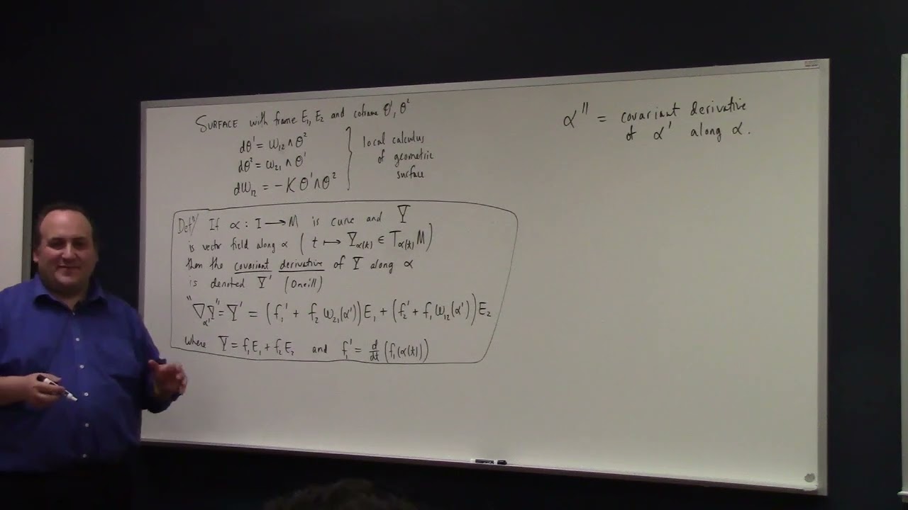
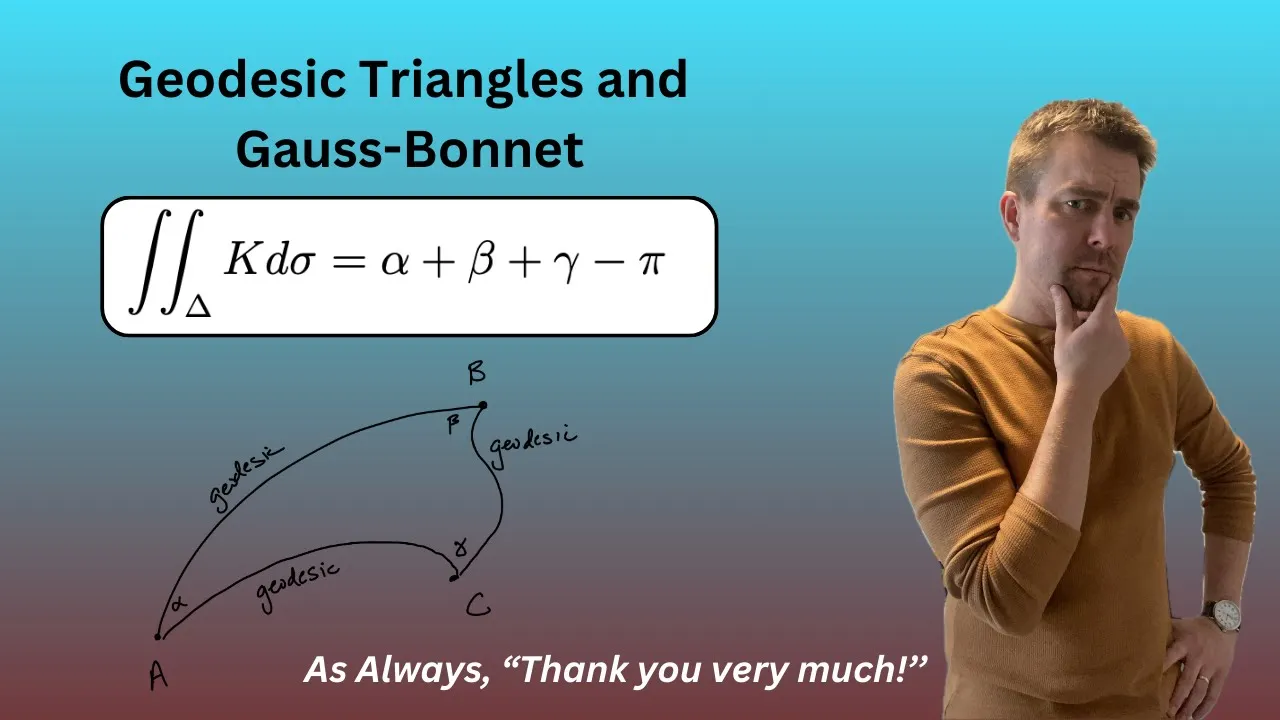
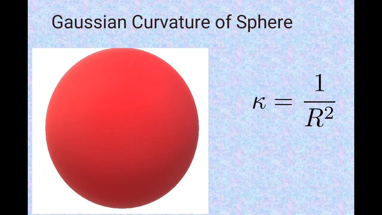








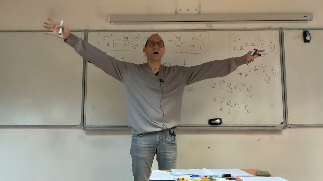

The Gauss-Bonnet Theorem states that for a compact oriented surface M with area form dM, the total Gaussian curvature is equal to 2π times the Euler characteristic of the surface: ∫∫_M K dM = 2πχ(M). This profound result connects purely geometric quantities (Gaussian curvature) to purely topological invariants (Euler characteristic), demonstrating that the integral of curvature over a surface depends only on its topology, not on its specific geometric shape.
Gauss Bonnet Theorem Proof | Differential Geometry Lecture 27
Added:Understanding of Gaussian curvature and geodesic curvature of curves on surfaces.
Basic topological invariants, specifically the Euler characteristic of a surface and the concept of triangulation.
Familiarity with vector fields, differential forms, and integration on manifolds, particularly Stokes' Theorem.
The Local Gauss-Bonnet Theorem, which connects the integral of Gaussian curvature over a geodesic triangle to its interior angles.
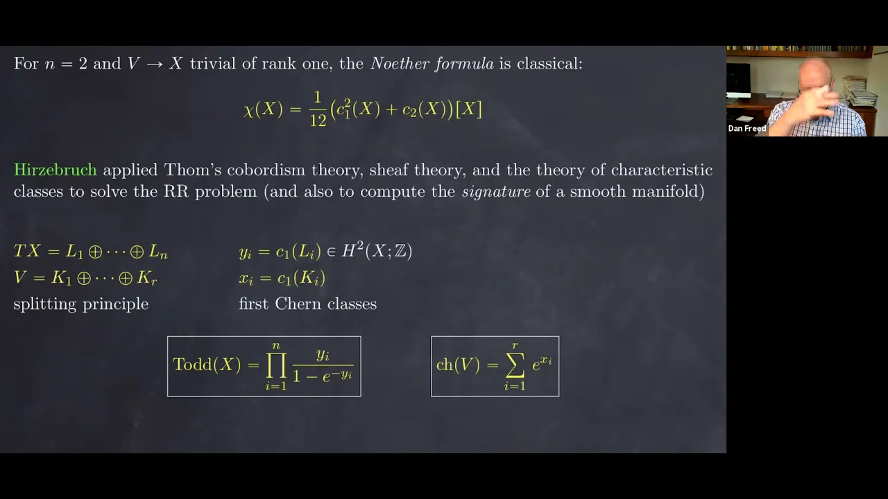
The Generalized Chern-Gauss-Bonnet Theorem, which extends the relation between curvature and topology to higher-dimensional Riemannian manifolds.
The Atiyah-Singer Index Theorem, a monumental result in modern mathematics that generalizes Gauss-Bonnet to elliptic differential operators.
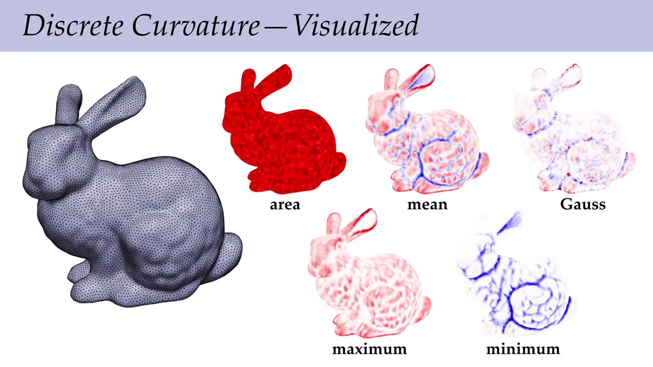
Applications in discrete differential geometry, such as computing discrete curvature and parameterizing 3D polygonal meshes in computer graphics.
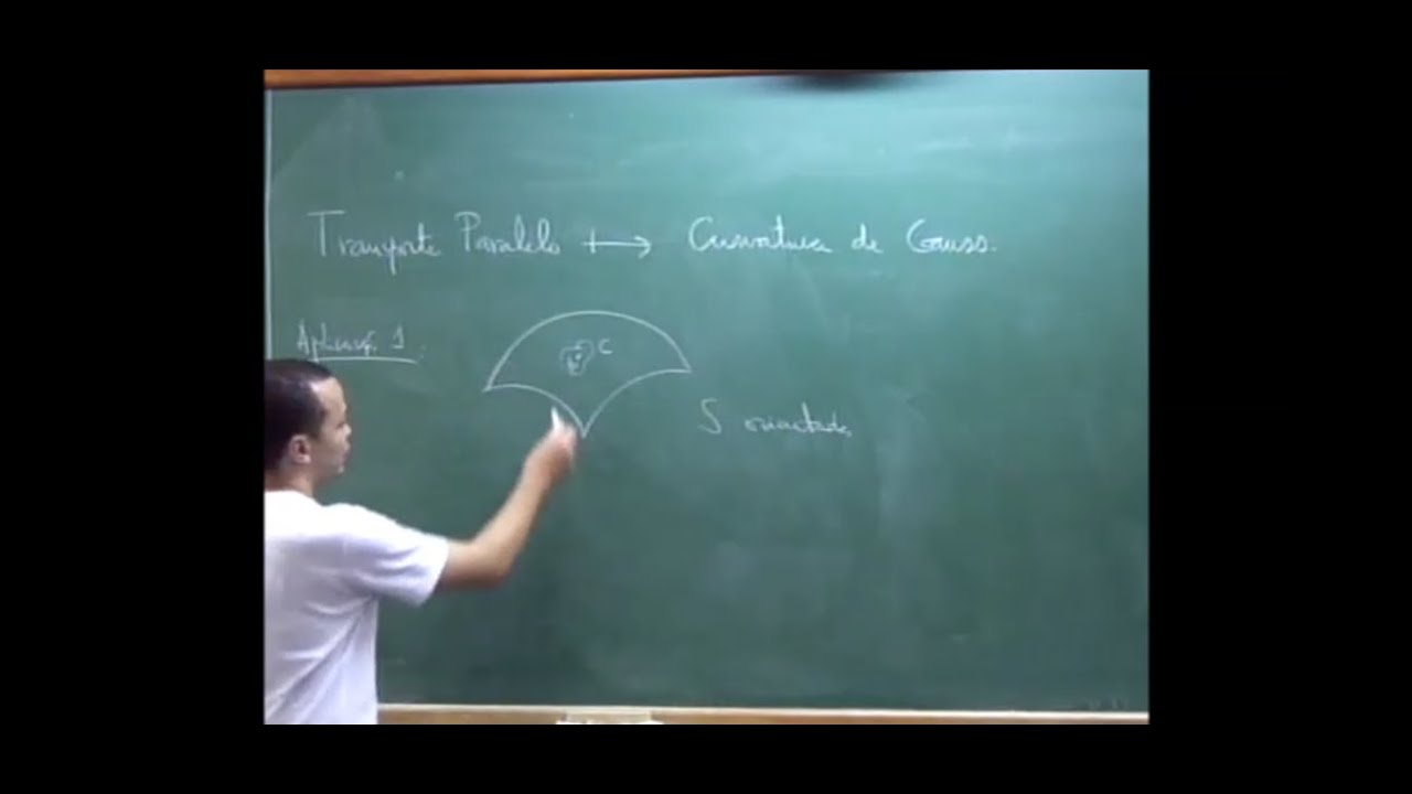
The study of Holonomy and parallel transport, analyzing how geometric phases relate to curvature integrals over closed loops.
7.9K views50likes55:55Original Release: 2015-08-07
All right. So, lecture 27 is on the Gaus Benet theorem. We're going to look at a at least a sketch of the proof. Um, it's partial because we will be relying on some results from um from topology uh which we will not prove. Um so, and and also I would mention that um the argument I give here is is more or less what's in O'Neal. Um I think there if you if you want to see something that's a little bit more uh detailed there's a nice chapter in John Lee's Romanian manifolds book um which has some some arguments due to Hoff and also contains a generalization of the theorem um due to Hoff and Shern and then also there's a a book in it's either written or in the process of being written by um Lena Chiffron um Shiffren I'm probably mispronouncing her um which is at the moment at least available as freely as a PDF. It has a pretty pretty detailed um proof of some of the things we're going through in here. So there's there's lots out there um in addition to these um well-known arguments I'm showing you here.
Anyway, so um if you have a regular curve from AB to M suppose it's you know regular again um and an oriented geometric surface m the total geodessic curvature of alpha is by definition the integral over alpha of the geodessic curvature with respect to arc length right so what that means is that um we integrate from s of a to s of b the geodessic curvature parameterized by s oft and times the dst dt Um so I suppose we have not assumed an arclength parameterization here. I mean dst the speed could be um doesn't have to be unity. Now a good example of this is for you know the circle in the plane.
Um so here if I um give it the arklength parameterization basically divide by the radius there's that gives me unit speed there's the unit tangent the um you know so you're working in the fren so working with two dimensional vectors I rotate the thing 90° out pops this this gadget right here there's your your fren normal right and then so the geodessic curvature is just given by the um inner product of t and t prime and n right um I mean here the metric is the inner product okay so whatever and out pop sin^ square plus cosine^ squ as usual and so we get 1 / r is the geodessic curvature all right so while geodessic curvature and frenic curvature are in general different um when they do match up they match Of course again the geodessic curvature could be negative whereas the fren curvature is essentially by construction positive.
All right so now I got that out of the system we integrate 1 / r from 0 to 2 pi r and we get rs cancelling and we get 2 pi a counterclockwise oriented circle in the uklidian plane um has total geodessic curvature of 2 pi. In fact, this is proved in in Lee's book following Hop for a so-called curved polygon in the plane. His chapter starts with a proof of that. It's pretty interesting interesting stuff. Um, sorry, I'll stop advertising Lee's Romanian manifolds book, but it is a nice book. Anyway, once if you were to do clockwise on the other hand, you pick up a minus. All right? Because if you if you go clockwise the other direction the um the normal I think you still let's see if I can picture it. So this excuse me try to draw them both where you can see them. So here's the that's the counterclockwise right? So if I was to have a clockwise circle stupid white out it's going to smudge. Oh well. Um the tangent would point Wait a minute.
Is that That's counterclockwise.
Yeah, this is clock I I forget which way is clockwise, which way is not clockwise. This would be clockwise. Um so basically that would amount to you know we could think of replacing the arguments with minus the arguments but basically that just makes it s cosine.
All right. And so when you rotate you end up with I think minus cosine um plus sign minus cosine plus sign puts the normal out here for the clockwise.
So that would be the difference and that's why the geodessic curvature would be negative because the circle is falling away from the tangent. So this is this would be the the geodessic curvature less than zero. Of course this is geodessic curvature positive as we just calculated but otherwise the calculation would go through the same and you'd get minus 2 pi. All right. Um so as I was mentioning um this is proof for an arbitrary curved polygon uh in in Lee's uh book again result due to hop. All right. Correlary 4.6 we looked at last time was that the the geodessic curvature is related to the angle um between E1 and the velocity as follows. So it's just dds plus the one two connection form acting on the velocity of a unit speed curve beta. So you look at this and you integrate and out pops this this wonderful wonderful formula. Um so that the integral the the the so-called total geodessic curvature around alpha it's the change in the angle along the curve plus the integral of the one two connection form along alpha. All right for a regular curve segment. All right and the proof of that is really just integration of that lema we proved last time. Here's the proof. Uh so integral of cappa gds is by definition we take the geodessic curvature evaluated at the airplane function multiply by the speed s of 8 sv but um by you substitution that's the same as this right but then the um the total the geodessic curvature is given by dds plus omega2 of alpha prime we proved last time and I mean alpha beta I'm using Um what was alpha? Alpha was a regular curve segment.
I perhaps should have a beta prime here to to um to denote the um the arkline 3 parameterization of the original regular curve.
So, but if you can forgive me that notational di uh discretion um we have this but then of course the integral well fundamental the calculus integral of total rate of change is the total change and of course this is just the integral of the one two connection form along the curve and there you have it now this is I mean honestly this lema I mean I'm I'm close to saying this lema is the Gaus Benet theorem I mean it's well it's not quite accurate it's this is important though I mean this the the nuts and bolts of what most of what we do follows from this.
Anyway, um so continuing suppose we have um a one to one regular map from um from some you know subset of the plane to M and um this means that there is a ra which contains r which is open and x is regular on the extension to art. So r could be closed right. So if we we talked about regularity on a closed set that means that you can extend to an open set on which it's regular as we defined at the start and then then we return we've now returned to the discussion of two segments which we had set forth in a previous chapter. So here's your here's your uh your two segment and we do this funny thing which is really smart. Um, I mean, this is actually how I I try to encourage calculus 3 students to calculate because honestly, I mean, yeah, Green's theorem and other things are set up for counterclockwise oriented curves, right?
But there's just something like intrinsically error inducing of using opposite orientations on cartisian uh coordinate parameterized curves. So, well, I mean, to get the counterclockwise orientation, you maybe would want to use minus gamma and minus delta there, you know. Um but don't we make them you know left to right and down to up for delta beta and gamma alpha respective and so that gives us the the the the two so-called two segment which is like a curved square or curved rectangle rather. Um, it's actually a rectangle over here in the parameter space, but then the patch packs moves it up here or parameterization moves it up to this curved curved rectangle. And the boundary of x is alpha plus beta minus gamma minus delta because alpha and beta are going in the right way to go counterclockwise around the rectangle.
But then of course delta and gamma need to be reversed. All right, this is this notation is not it's not pointwise addition here. We're talking about the addition which is curve like the curve following addition. So there's this this is a slick notation for the concatenation of curves into a into a larger curve. I don't think I ever made that explicit and yet I hope you understood it.
There are other places and other times where making it explicit would be worthwhile. Specifically if we were getting into the nuts and bolts of homatopy I would want to get into that but that's not here. So the natural induced orientation of the boundary makes the edge on your left while you walk on the top of M. Let me just give you the picture again here. So if you imagine walking around this, this is M by the way.
And you know this is this is the top the top of M, right?
Um although I my my picture is just a picture. It's not you know um fundamental this surface could be inside you know 20x 20 matrices it could be a particular surface in 20 x 20 matrices I mean whatever this is an abstract geometric surface all right but um that said um you know there is is we also assuming well since we're working with x we can we can orient it use we can use the patch at least orient this this little two segment. All right. Now or I I should say we can use dm to orient it anyway. So let me stop move along here. So definition X from R to M be a two segment M. The closed rectangle R um from you know AB cross CD um has edge curves given by alpha beta gamma delta which in particular are so for alpha you let U vary you freeze C.
Um for for beta you let Vary you freeze um the U. and gamma we take u as a variable we freeze d right delta we freeze the u variable at a and we let v vary so if you go back to the the picture I just had on the previous slide it's these make sense if you look at it right so like alpha and gamma both have the same parameter froze and beta and delta both have the same parameter froze uh as you can see over here they're they're pre-im images.
Um, you know, alpha has v froze and then u varies and same for for for gamma but beta and delta have v as the variables which is what we wrote down here. All right. So just a little bit back from chapter 4 just reminding you guys.
So that said alpha plus beta minus gamma minus delta is a simple closed curve on the boundary. Well, not quite accurate. This is the concatenation of um these three these four curve segments. Simple closed curve, but it's not you know with stopping points. Not not quite, you know, not quite not quite.
We have vertices. All right. we have the the uh the joining points to the curves. So what's the total geodessic curvature at the boundary of x? I mean this is true in terms of the point set. All right that's definitely true. But the thing is when you're calculating the total geodessic curvature of that boundary um you know the corners matter. All right. If it was single curve, we wouldn't have to wor worry about it. But the corners matter here because the, you know, the angle can change um at those corners, right? That angle between E1 and the um tangent to the curve. So, what we're going to have is we're going to have the integral around the boundary is equal to that that plus that plus that. Um, and I don't think that's quite accurate.
Plus what?
quarter terms, right?
Plus quarter terms.
All right.
Now, here's a picture, but I mean, I'm just I'm just getting as far as the um the boundary of x goes, it's this plus this plus this plus this.
And then the minus pulls out because you know um because we're this isn't oriented um well because the geodessic curvature flips signs uh when you when you reverse the orientation of the um you know the curve curve segment more specifically uh you say oh wait wait wait I remember from calculus 3 that the arklength integral is in it doesn't care about if you reverse the orientation it doesn't doesn't change signs.
Well, that is true, but we're not integrating. This this geodessic curvature is not an innocent bystandard.
When you reverse the orientation of the curve, it it it reverses its sign as we just saw with our circle example at the start of this lecture. So, that's why the minuses pull out because the geodessic curvature flips. Now, excuse me, plus the corner terms, right?
And those corner terms is what we're going to talk about next. Um, here's a picture. That's the start of it. All right? Maybe this is all of it, actually.
Um so your your your you know your curved rectangle could look something like this. And if I want to calculate the um the total geodessic curvature um of like this purple I've tried to draw like a purple curve. So you can think about it like what's the total geodessic curvature of that with these rounded corners. And then as as they kind of in the limit get to the corners they have to pick they have it has to match what you'd get from integrating the geodessic curvature along alpha beta minus gamma minus delta respectively and you'd also have to add in these these other terms here from from the turning of those um let's see here so again if I if I just take well I guess Sorry, I um it's a question of notation mostly, but I shouldn't have crossed this out earlier. I'm sorry. Me scratch that. The reason for that is he really does mean the boundary of X is just the union of these two segments. But um the thing is we're going to want to realize this as the boundary of a um you know a simply connected region in a bit. And so there I need a I need a nice I I need a nice boundary curve and this is not that. I need this sort of curvy one in order to make a connection with theorem later.
All right. I'm sorry. I just it's no notational that's getting me here. But um so he says C is the boundary of X with the corners cut. And so the integral around C is not equal to the integral around the boundary of X because why? Because it neglects the this this neglects the turning. All right, which you would have with the little purple curve. Um so let XR be pictured above. The vertices are P1, P2, P3, P4. And the exterior angle epsilon J of X at PJ. So epsilon 2 at P2 3 at D3 and so forth. Um they're derived from the edge curves in the order of occurrence. And likewise the internal the internal angle is I believe supplementary to epsilon j right the sum of the internal and the external area external angles is pi. So like the internal angle would be like here for this one. The internal angle would be if it extended that would be like here and so forth. The internal angle here would be be like in here and the internal angle here would be like there.
Oh, I think I was just I'm sorry. I was off the off the map. Goodness gracious.
Sorry about that. Try that again. So, the internal angle, if I extend this back, the internal angle would be like in here. If I was to extend this back, you can see the internal angle in there.
If I extend this back, the internal angle's in here. Extend this back, the internal angle's like right in there.
External plus internal, external plus internal, external plus internal, external plus internal. all come out to pi. All right. So, well, here's some formulas that connect them, right? Um, so now depending on the picture here, you know, we either have um acute or obtuse angles, right? So, like epsilon 1.
Well, I have epsilon 2 equals to theta 2. What? What? Why do I say that? I'm sorry, guys. What's theta?
All right. Well, I I say look over. I better follow my own advice. Um, all right. So, I say, oh, oh, I'm sorry.
Here it is. The coordinate angle theta is between 0 and pi. And it's the angle from xu to xv for these patches. All right. So, like theta here, theta 3. So if xu now which one is xu and which one's xv it depends on which curve we're looking at right each remember these are either u or v parameter curves so it's just a matter of bookkeeping but like this one is a v parameter curve and and xv points that direction this is a u parameter curve right and so xu points that one that way but of course minus the curve points this way and um so the angle the uh the turning angle is the angle between where it was going to and where it's going you know where it was going from and where it's going to. So this is the epsilon 3 theta 3 is defined to be the angle between xu and xv and the relation between the theta and the exterior angles different at different vertices. Um so for example here the sum of them is obviously pi right but if you look at similar pictures to prove the remaining assertions well let's do that for example um over here at the other on the other edge of the rectangle you have the um here's where xv would be pointing xu is pointing that way right um as my picture is drawn now epsilon 4 is over here and theta 4 is over there How are they related? Well, they're equal, right? Because they're these are that's actually a line and that's actually a line. Just it's kind of got a little bit bent in my picture, but it it it's supposed to be a line. So these are these are equal by elementary geometry, right?
Those alternate interior angles or something. And um so similarly you can prove as I was mentioning over here that epsilon 1 is equal to you know p<unk> - theta 1 epsilon 3 is p<unk> - theta 3 but at those other two edges because of basically what I just we just saw epsilon 2 the exterior angle is equal to the angle between xu and xv um in those cases. So that said, sorry there's a lot of lot of things going together here, but once it comes together, you'll you'll like what we find. So we have a regular 1:12 segment in a geometric surface m dm the area form all this notation put together.
If we integrate um KDM, Isaac, buddy, got to play quiet.
Okay, thanks. If we integrate KDM over this two segment like that, well, it's equal to the integral um over the boundary of the two segment, right?
Plus these exterior angles and that all has to al together has to be equal to 2 pi. This is the um Gauss Bonet theorem with exterior angles. All right.
Now here epsilon j is exterior angle of vertex pj as we defined.
So the gospo this is gosp formula with exterior angles in terms of the interior angles. You can also rewrite it as follows. The integral of this is the total gaussian curvature of the two segment. Right? This is the total geodessic curvature of the boundary. And that has to be equal to the sum of the exterior interior angles minus 2 pi. All right. Um, now we have sums of four angles because we're working with rectangles, right? There are similar theorems that you could prove for a triangle where you'd have the sum of three exterior angles and the sum of three interior angles. And I think you'd I I think you end up with pi and minus pi instead. But I should not I I I haven't that's I'm speculating. I I haven't thought through the details there. I'm just All right. Um, sorry. So here's the proof. Let me stick on stick on what we're doing. So based on the frame field associated to X in particular um for this two segment we can set up the frame E1 which is XU normalized and then E2 is J on E1 and such and and that's chosen such that that DM is E1 DM on E1 and E2 is equal to one. All right. So we're choosing the positively oriented frame and then we recall the second structural equation.
And the second structural equation defined the Gaussian curvature for us.
In particular, d omega12 is equal to minus kdm.
But on the other hand, we also know that d omega12 plus kdm equal to 0 by algebra. So great. Then what can we do?
Well, we can integrate and the integral of 0 0. But so we have the integral of d omega12 /x and the integral of cap galsian curvature um over the the area form of the whole two segment but now we use stokes theorem well generalized stokes theorem I suppose which we have not proved but you could prove uh anyway so generalized stokes theorem says the integral of the differential is the over the over the bulk is the integral of excuse me the integral of the exterior derivative of a form over the bulk is equal to the integral of the form over the boundary.
So there you there I mean there we have it.
But on the other hand the relation between the integral of this form over the boundary and um and the interior angles or exterior angles and total geodessic curvature is somewhat complicated, right?
And so by the lema on the next page, this just works out to integral over the boundary of the geodessic curvature plus these turning angles, the exterior angles bob - 2 pi by the lema on the next page.
And that is the Gaus Ben theorem with exterior angles.
All right. Now, so here's the here's the lema.
The integral over the boundary of the one two connection form is equal to the integral of the um you know the uh words the the geodessic curvature over the boundary of x plus the turning angles here minus 2 pi. Now, so to break up this integral, I've got this plus that minus that minus that.
Um, so what do we got here?
The integral.
And then for each one of these, we go back to that um lema proposition theorem. I forget what we called it in the last lecture where we showed that the integral of the connection form along a curve was the difference in the fee angle plus the integral of the the geodessic curvature along along the uh along the curve.
Right? And so that's the thing is this is non-trivial for um for these for these curve segments, right? And so let's see here. So I seem to be arguing that f of b is equal to f of a here.
Not sure why this is always zero along alpha.
Oh, that has to do with the definition, right? V is the angle between E1 and alpha. But when when E1 is just alpha prime normalized, of course, the angle is the same because the angle is zero essentially by definition of V and by E1. All right. Okay. Duh. Sorry, I get so much notation floating around I forget what's what. And then I talk myself into using theorems I don't need to use. I hope you can sort through my um my comments here to make sense of it.
Anyway, so if we integrate along beta again using the proposition from last lecture, we get f of c minus f of d.
Now, this time beta is based on the v parameterization. So there's no reason that this angle and that angle have to be the same. But um these these are um those angles are the thetas, right?
because it's the angle between E1 and the tangent to beta. But that's the angle between XV and XU, the partial velocities of the patch, which is what we called theta, which by the way is the difference between pi and the third exterior angle. And um for for this one, and then the other one is on the flip side, the theta was just E2. So lo and behold, we get E2 plus E3 minus pi.
Sorting through the details there.
Here's some attempts at a picture. So E1 E1 E1, right? And so this is the angle to start with. That's the angle to end with.
And um let's see. This this picture could be improved slightly if I put in if I actually put in which which vertex we're at.
Let me do that.
I think the numbering hopefully I'm getting.
So beta went from P2 down here up to P3 up here, right?
Whereas alpha goes from P1 to alpha went from P1 to P2, right?
And then continuing the third one goes from where did we go from? Come from P3 over to P4.
But this time the angle is always pi I believe. Let's see here. Um yeah minus is minus gamma is opposite the E1 direction. Right? So these are equal. So we just get the integral.
We just get the integral of the geodessic curvature along gamma for the integral of the one two connection form in that case.
All right, one more to go for the fourth curve segment we have going from P4 back to P1.
Finally completed the loop. I'll just draw P1 down here. I'm not going to try to draw P4 up there. It's too cluttered already. Um so there of course we have the integral along delta of the geodessic curvature but we also have the difference in the fee angle which the fee uh up here is is is like this and so it's pi minus epsilon 1. Up here we have fd is epsilon 4. So we end up with pi minus epsilon 1 minus epsilon 4.
So then when you put all four of these things together and add them out pops the really cool thing which is that the integral over the boundary of x of the one two connection form is this plus that minus that minus that but you get a minus pi here. You get another one here.
So you got a total of minus 2 pi and epsilon 1 plus epsilon 2 plus epsilon 3 plus epsilon 4. And there you have it.
That's the lema that we used to establish Gauspa theorem with exterior angles.
So you know it's kind of overwhelming if you just look at it but if you actually sort through the details there's nothing here that is really beyond anyone's comprehension. It's just one step at a time. It's all not that hard to understand really now. So that I think but goodness the Gaussman theorem usually also involves the that that's part of the Gaussman theorem really I've been calling it the Gaussman theorem I mean that's that's the differential geometry side of the Gaussman aumore right this everything we did was just geometric about angles as it relates to a particular uh total Gaussian curvature right so this just to be more specific as I'm saying this so I've called this the Gausman theorem um and so do other But the other thing that gets called the gaspay theorem has a connection to something else called the oiler characteristic. Now we haven't talked about that yet here. This this this theorem just involves total curvature geodessic curvature um these particular turning angles at the edges of the two segment right um so I just again this is totally a geometric discussion right now what follows is topological so um you know one of the fundamental programs in topology is triangularization or rect rectal rectangularization of surfaces it turns out by making images of triangles or rectangles on an abstract surface. You can discover things about its it its topology. Um it's a way of detecting holes and all sorts of things. Um so this is a somewhat old story. I think it you know Oiler did some those bridges of Cronisburg and but it's it's you know really coming into it in the last maybe 150 years or so.
So first let's just talk about the idea of rectangularization. The idea of a rectangularization is you take your surface and like fill it up fill it with some um with some curved rectangles some some two segments as it were and they have to like completely you know fill the whole space and cover it. Um you know obviously this isn't unique. I could take one of these and like cut another one and add more rectangles right. Um, this door is a joke specific to the first time I taught the course because uh, one of my students got in this ridiculous argument with his roommate about a door and I uh, I just wanted to bring it up again because it was a sore point. Anyway, stupid jokes aside, every compact surface has a rectangular decomposition.
This is a special kind of paving, of course. Um, now the proof is by scissors on page 369.
um more serious answer is some of these these triangularizations or or rectangular like rectangularizations are established in deeper books on topology.
Uh Lee mentions I think Massiey's algebraic topology book or what was it?
Sir, what's the other reference? Um Allan Seridaskki's introduction to topology and homotopy um 1992. That's another place where you can find I mean there's probably lots of books that have these things proved but we won't. The point is there is a rectangularization for a compact surface. Now let's talk a little bit about the difference between um you know topology and differential geometry. So topology is concerned with what are the open sets and also what are you know um what are the continuous maps a map is said to be continuous in topology if it has the property that the inverse image of open sets is open. And so in topology you can ask whether two spaces that both have topologies which just means that there's a definition for what's open on those two spaces. And you can compare the not the uh you know the sense of you know open sets on one versus open sets on another. If you have a bjection between these two sets, right? And that bjection um is continuous in the sense that it takes open sets here, inverse image open sets here. And if that bjection also has a um inverse function which is likewise continuous, uh if you have both of those things, then that bjection is said to be a homeomorphism. Homeomorphisms are the uh maps in the theory of topology which preserve topological structure. So a topological invariant is one which is preserved by homeomorphisms. Just like us we have talked about um you know well we didn't talk too much about this but diffomorphisms are smooth mappings with smooth inverse you know smooth is is much strict is is a more complicated thing perhaps than than than continuous right so diffomorphism is bjection that is smooth with smooth inverse and still more still different than that we've also talked about isometries between spaces where there you have a bjection Right. And the um the the bjection preserves the the metric from the one surface to the other. Right? So it preserves you know this this notions of distance and angle because we've just talked about two dimensional isometries.
Right? Of course these these these comments have generalizations.
So you've got these these uh you know these different notions um you know isometry difforphism homeomorphism and you know what are the connections? Can you get from here to here? Can you get from there to there? What what what's the bridge between these worlds? Is there a bridge between these worlds? So it is true that diffomorphism implies homeomorphism.
Um because if it's smooth it's continuous. Right? So back to calculus one again, right? Differentiable implies continuous. However, continuous does not imply differentiable and that's why we can't reverse this arrow. So, but that said generally the converse is false. A homeomorphism does not imply that f is a diffmorphism. That's why the following result is in some sense shocking. In dimension two, M is homeomorphic to N.
All right, surfaces if and only if M and N are difforphic.
That's very very nice.
Now that's proved. I don't know if we prove that here. I think that's proved in topology books, but anyway, we we will we will see evidence of that.
Anyway, um all right. Like I said, we'll have to I'm not sure that's proved in the text.
I still not sure. I kind of think not.
Um so, theorem 6.6 six.
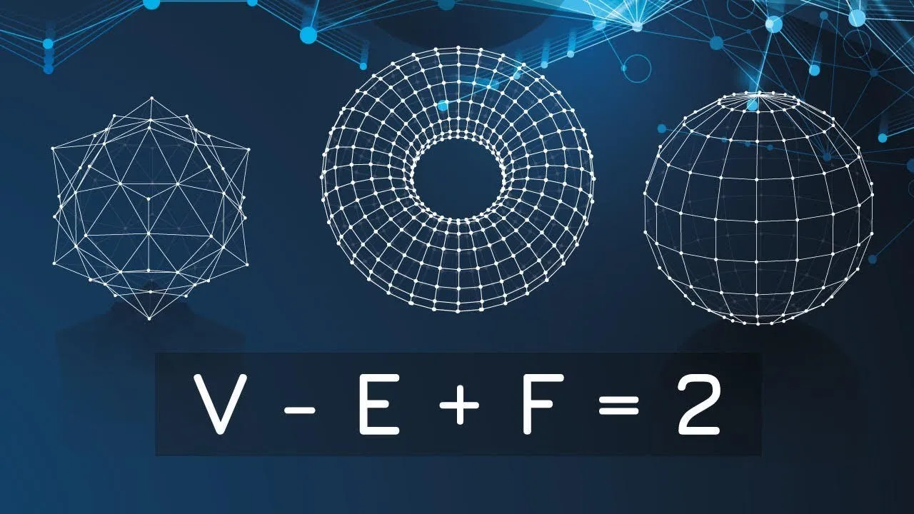
Now, this is a theorem we're borrowing from topology. All right? If D is a as a rectangular decomposition of M, a compact surface, let um new E and F be the number of vertices. I'm going to say V. Let V, E, and F be the number of vertices, edges, and faces in D. The integer V minus E plus F is the same for all such decompositions. Moreover, this integer is called the oiler characteristic.
All right. Um, so the oiler characteristic of M is V minus E plus F.
Maybe uh maybe after this I'll add a little video showing you how to how to do this for a triangularization of a sphere. I don't have it in these notes.
I may have some pictures here, but maybe I'll do some arts and crafts here after this after this lecture to add something here. Anyway, the proof is given in topology, but this equally well applies to polygonal decompositions. I said see the handout from le text. Well, how about just go buy a copy of le text and read it. But um so the sphere for example has oiler characteristic two one. Um, basically you can just take the you can imagine in your mind's eye taking this tetrahedrin right and just kind of blowing it up into these curved tetrahedrin like curved triangles that um, you know fill out the sphere the edge of the sphere.
And so that gives you a triangularization of the sphere. It has it has four vertices.
It has six edges. 1 2 3 four five the one in the back six. and it has four faces. So 4 - 6 + 4 is 2. That's one um you know polyhedral approxim approximate of the sphere triangularization.
rectangularization.
Um rectangularization similarly you can imagine sticking inscribing this rectangle or cube inside a sphere and then just imagine those edges kind of blowing up to f fill the edge of the sphere. Um now that that process obviously does not preserve lengths and angles, right? This is not a not a geometric process I'm describing.
It's a topological process because it's we're talking about um you know a distortion of geometry in part in particular in the sense of distances and angles being distorted but um anyway you can imagine in your mind's eye blowing it up and getting a sphere. So this gives you rectangularization and then if you do the counting here we have eight vertices we got 12 edges we got six faces it still works out that two. Now, of course, that is not a proof of the invariance of the oiler characterist characteristic across different possible rectangularizations of the sphere, but it does make us feel good about it. All right. All right.
So, the Taurus um has oiler characteristic of zero. I say I don't see it yet. I think I have maybe maybe that's one I should do in the in the separate video then that would add some goodness um to these notes. All right. So another thing we can do is we can add a handle to a compact surface and that will reduce the oiler characteristic by two. So adding a handle is like pasting a donut on something else. So, here's your here's your initial surface. Um, and then glue on this this this doughut like that. And the um so if you think about it, if you believe that the Taurus has oiler characteristic zero, the net um sum of you know V minus E plus F is zero for this thing, right? And in the process of gluing it, what happens is you delete a face from from both, right?
And that's let's see here. You delete a face from both. What about edges?
I guess you still have the same number of edges and vertices as you did before. Not sure. I believe that.
Seems like you're adding I think you're adding goodness gracious I want to say I I say on M you're adding four vertices and four edges but V minus E is 4 - 4 is zero. So yeah. Yeah, that makes sense. So basically, you're just losing the two faces and the edges and vertices even out because you have plus vertices and minus edges. So the oiler characteristic of the um surface with the with the handle glued on it is equal to the original earlier characteristic minus 2, which is kind of cool.
And that gives us this theorem.
If m is a compact connected orientable surface, there's a unique integer h greater than equal to zero such that the surface is difforphic to a sphere with h handles with with h donuts glued onto it. All right, a sphere with h handles attached.
Um it's a theorem.
Now a correlary to that theorem is that compact orientable surfaces m and n have the same oiler characteristic if and only if they're diomorphic.
So if the oiler characteristic of m is equal to the oiler characteristic of n that means that m and n have the same number of handles then by theorem 6.8 m&m are difforphic. All right.
So getting back to Gaus Ben the full version of it. The total G gaussian curvature of M of a compact orientable geometric surface M is 2 pi. All right times its oiler characteristic.
Whoa.
You're like what happened to the what happened to the geodessic curvature and and the exterior angles? Why? Where?
It's now it's the oiler characteristic.
Right? This is this is a really really beautiful beautiful result because it links right the geometric the totally geometric quantity of the total Gaussian curvature of the surface to this intrinsically topological invariant of the oiler characteristic. So here here we have worlds collecting as it were.
All right. um the orientation of M by the area form DM and we'll let D be the rectangular decomposition of M whose rectangles are consistently oriented with DM. That means that D is an oriented paving as discussed and defined in section 6.7 page 302. By definition, the total curvature of M is we have to integrate over the paving, right? You total curvature of each um you know each tile in the paving if you like and um where F is the number of faces, right?
So the number of faces which is the number of rectangles here.
Now you apply the Gauss Benet theorem the Gauss Benet formula probably should have been calling it Gausp formula that's why I'm confused. Ah words words words words words words words words words words words words words words words words words words so anyway the gasp I've called it theorem but it's really the formula the gals a formula to each face and then we have what we have the integral of kdm over the face is equal to this since I've written it in terms of the interior angles right and but every face is adjacent to another face and so the boundaries are are are overlapping in particular we have that the integral over alpha i plus the integral of alpha j um I think that's supposed to be I've lost my kappa the geodessic curvatures um you know that cancel so because of the way the I hopefully have a picture oh it's the same kind of argument that we use in calculus 3 to prove um you know like the various theorems for for surface integrals where we we break it up into pieces and then on the separate pieces you have you know counterclockwise orientations on each each piece. So oh stink do I have room to draw something here?
So like there's there's two cells, two faces, right? And so they're both they have to be consistently oriented like that, right? So on the one side you're going this way, right? But on the other side, you're coming when you hit that leg that that boundary curve goes that way. So they're when they're in interior um these interior legs, these interior um edges, they meet up with opposite orientations. So these integrals cancel out along those interior um cancelling edges.
That's why you end up with like integrals over the boundary of um surfaces because these interior terms tend to cancel. Anyway, okay, getting back to the proof. So all of the integrals over the boundary of these geodessic curvatures cancel as we integrate over all faces.
Um and moreover there there is no external curve right we're talking about a uh a compact orientable geometric surface. Sometimes this is called a closed uh surface.
There there is there's no edge. All right there's u just interior face.
There's only interior edges is my point.
All right. So the fact that these cancel means that this these terms completely drop out. Moreover, the um the sum of the interior angles is 2 pi at each of the each of the vertices. Um which makes sense if you think about it. Um thus by you know applying the Gaussman formula we have the integral of the total the total Gaussian curvature is the sum over the number of faces of - 2<unk>i plus the sum of the interior angles but of course the sum of a constant f* is just you know that constant time f. So that gives us a minus 2 pi f and then we get sum i = 1 to f of the interior angles of the i face.
All right. But the interior angles of the i face is just given to us. I say that that's 2 pi v. Why is that? Well, the claim Oh, sorry. Why is that 2 pi v? Let me just stop and think for a minute here.
Why should the sum of the interior angles of the i face work out to 2 pi * v?
Now f is the number of faces, right?
v is the what's v again? V is the number of vertices.
H curses.
Why is that V [Applause] H?
Maybe if we look at the examples on the next page, it'll become clear. Let's see here.
So here for example is a uh you know rectangularization of a of a rectangle.
Um so the claim is that 4f is equal to 2e.
That doesn't help me see why that sum of interior angles for the i face was was 2 pi v.
Huh.
What's the relation between number of faces and number of vertices?
Um, each face gives you how many vertices?
Well, it gives you four uh vertices, right?
But some of those are shared, right?
So, I mean, you can't just say that there's um man, why is that 2 pi v?
Goodness gracious. It must be something simple I'm just missing.
Oh, man. All right. All right. Well, I I'm going to leave that as at the moment an exercise for the reader.
I must I must go on here.
Uh this is something you can check for different uh rectangularizations.
Four * f is equal to 2 * e. Uh so let's see here. 4 * f is 2 * number of faces.
Four * the number of faces is equal to two times the number of edges.
And you can you can check it out. that it works for this example, but that that's generally true. So, a proof continued. I more often than not when I get stuck on something like this, the answer to what I'm stuck on is in the next next little bit, and I just forgot. But anyway, here we go. Each face has four edges, but each edge belongs to two faces. Thus, 4F counts E twice. That is 4F equals to 2E.
All right, that's from from O'Neal's O'Neal's page 374. All right, so the oiler characteristic was defined to be V minus E plus F. But that works out to V minus F because this gives us that minus F is equal to F minus E by algebra. And so F minus E is just minus F.
So which which does actually kind of make you wonder like oh I'm sorry this is for rectangular decompositions you know if you look at other other books which have proof in terms of triangularizations these arguments these these little details here get they get distorted into other um little combinatorial you know factoids like like here 4 f= 2 a right anyway returning to the total curvature is equal to 2 pi v minus f but that is the other characteristic so we get the total curvature total galsian curvature is 2 pi time * our other characteristic and I'm sorry I still have not explained why it is that the sum of the interior angles of the i face works out to v * 2 pi I mean what what is the sum of interior angles of a particular rectangle Well, that's p<unk> /2 + p<unk> / 2 plus p<unk> /2 plus p<unk> /2, I believe. So, it seems like you got um two pi interior angles for each face.
Um but he's 2 pi V. Man, I I am sorry. I I don't I don't see that. That's just me, though. I'm sure there's some obvious reason. Oh, and that brings us to applications of Gaus Benet, which is the next lecture. So, I'm going to stop here. I hope I made some sense. I'm sorry for the mangling of terminology. I think at the end of the lecture, you can see all of my transgressions. I called the gasp theorem, the gaspay formula. I mean vice versa. I should have said it was Gaspin formula back at the start of the lecture. And what was my other other abuse of terminology in here? Um the other thing was it really was the boundary of X. It wasn't not the boundary of X. It's just that to calculate the total um the total geodessic curvature you um excuse me to calculate the change in the connection form around the boundary you have to take into account the change of the uh change of the angle. So anyway, I will stop it
Up Next
22:59
Euler's Characteristic: Topology and Geometry Applications Explained
@zachstar
448.2K views•2019-09-13

4:43
Elliptic Curve Cryptography Explained: ECC, ECDSA, ECDH
@PracticalNetworking
28.5K views•2024-10-21

10:44
Fourier Series Introduction: The Big Idea Explained
@DrTrefor
387K views•2021-05-03

6:00
The Mathematical Impossibility of Accurate World Maps
@Vox
23.3M views•2016-12-02
Related Study Plans & Knowledge Roadmaps
Structured learning paths in Mathematics
mathematics
Tensor Calculus: Vectors to Riemann Curvature
01Mathematical Foundations: Linear Algebra & Calculus
02Covectors, Dual Spaces, and Tensor Basics
03The Metric Tensor and Index Gymnastics
+ 2 more learning modules
40h5 modules
Explore Roadmap
mathematics
Gödel's Incompleteness: Logic, Proofs & Limits
01Introduction to Formal Systems & Hilbert's Dream
02Set Theory, Cardinality, and Cantor's Diagonal Argument
03Arithmetization and Gödel Numbering
+ 2 more learning modules
14h5 modules
Explore Roadmap
mathematics
Galois Theory: Fields, Groups & Solvability
01Foundations of Abstract Algebra: Groups & Fields
02Polynomials & Field Extensions
03Splitting Fields & Symmetries
+ 2 more learning modules
24h5 modules
Explore Roadmap
mathematics
Non-Euclidean Geometry: Models & Geodesics
01Euclid's Fifth Postulate and the Birth of New Geometries
02Hyperbolic Space and the Poincaré Disk Model
03Geodesics: Defining Straight Lines in Curved Spaces
+ 2 more learning modules
15h5 modules
Explore Roadmap