This video demonstrates the quantitative validation of analytical methods used in quality control, covering key statistical parameters including Limit of Detection (LOD), which represents the lowest concentration of an analyte that can be reliably detected; Limit of Quantitation (LOQ), which indicates the lowest concentration that can be quantified with acceptable precision and accuracy; and Standard Deviation (SD), a measure of variability or dispersion in analytical data. The instructor explains how these parameters are calculated and applied to ensure the reliability and reproducibility of analytical results in laboratory settings.
QC Validation of Analytical Methods: LOD, LOQ & SD | Absorbance & Concentration
Added:Deep Dive
Understanding of the Beer-Lambert Law and the mathematical relationship between absorbance and solute concentration.

Loi BEER-LAMBERT : absorbance et concentration | 1ère spé | Chimie
506.3K
The Beer-Lambert Law states that for a given wavelength and solution thickness, the absorbance (A) of a diluted colored solution is directly proportional to its concentration (C). This relationship is mathematically expressed as A = εlc, where ε is the molar absorption coefficient (dependent on wavelength, solute nature, and solvent), l is the path length of the solution traversed (cuvette length), and C is the concentration in mol/L. The absorbance is a dimensionless quantity.
Click to watch →

Beer-lambert's law Derivation | Plots | Limitations | KTU-ENGINEERING CHEMISTRY ♦️ SPECTROSCOPY ♦️
24.4K
Beer-Lambert's Law states that the absorbance of light by a solution is directly proportional to the concentration of the absorbing species and the path length of light through the solution, expressed as A = εlc, where A is absorbance, ε is the molar absorptivity coefficient, l is the path length, and c is the concentration. This fundamental principle in spectroscopy allows quantitative determination of solute concentrations by measuring light absorption, with applications in chemistry, biology, and environmental science. The law assumes monochromatic light, homogeneous solutions, and no chemical interactions between absorbing species.
Click to watch →

UV Visible Spectroscopy || Principle || P 2 U 1 || Instrumental methods of analysis | Carewell Pharm
485.9K
The Beer-Lambert Law (A = εcl) mathematically describes absorbance relationships: A = absorbance, ε = molar absorptivity, c = concentration, l = path length. Absorbance increases with higher concentration (more particles to absorb light) and longer path length (light interacts with more particles). This linear relationship enables quantitative concentration determination by measuring absorbance at known wavelengths. The law provides the theoretical framework for all quantitative UV-visible spectroscopic analyses.
Click to watch →

BSc Semester - V | Chemistry | One Shot Marathon Class I Most Important Topics | PDUSU
6.7K
The Beer-Lambert Law describes the relationship between absorbance and concentration of a solution. The law states that absorbance (A) is directly proportional to the concentration (C) of the absorbing species and the path length (L) of the light through the sample. The mathematical form is: A = εLC, where ε is the molar absorptivity (a constant for a given substance at a specific wavelength). The law is fundamental in quantitative analysis using spectrophotometry.
Click to watch →

Espectrofotometria e a lei de Lambert–Beer
46.8K
The Beer-Lambert Law states that absorbance (A) is directly proportional to both the concentration (c) of the solute and the path length (L) of the light through the solution: A = ε × L × c, where ε (epsilon) is the molar absorptivity coefficient, which depends on the specific solute, the wavelength of light used, and the temperature. This linear relationship allows scientists to determine unknown concentrations by measuring absorbance at known wavelengths.
Click to watch →
Deep Dive
Basic statistical concepts, specifically how to calculate and interpret the mean, variance, and standard deviation of a dataset.

Complete Qualifier Stats 1 Oneshot | Week 1-4 | Notes Attached | Gen-Z IITian | BS Degree
426
Mean = sum of observations / number of observations. For grouped data: Mean = Σ(fi × xi) / Σfi, where xi is class mark. Adding a constant to all observations increases mean by that constant; multiplying by a constant multiplies mean by that constant. Variance = average of squared deviations from mean = Σ(xi - x̄)² / n (population) or n-1 (sample). Standard deviation = √variance. These measures describe the central tendency and spread of data.
Click to watch →

Statistics: Standard deviation | Descriptive statistics | Probability and Statistics | Khan Academy
2.3M
This segment covers three core statistical concepts essential for data analysis. The mean (μ for populations, x̄ for samples) represents the central tendency, calculated as the sum of data points divided by their count. Variance (σ² for populations, s² for samples) measures dispersion—the average squared distance from the mean. For populations, divide by N; for unbiased sample estimates, divide by (n-1). Standard deviation (σ or s) is the square root of variance, returning to original measurement units for better interpretability. These measures together describe both the central location and spread of a dataset.
Click to watch →

HOW TO USE CALCULATOR TO CALCULATE FOR MEAN, STANDARD DEVIATION, VARIANCE AND ETC
15.8K
To calculate statistical measures: Press SHIFT then 1 (STAT), select 4 (VAR). For mean (x̄), select option 2. For population standard deviation (σ), select option 3. For sample standard deviation (s), select option 4. To calculate variance, square the standard deviation by pressing the x² button. The mean represents the average, while standard deviation measures data dispersion. Population statistics use σ, while sample statistics use s.
Click to watch →
 Matemática A, B e MACS - Programa Velho e Novo (1 e 2 variáveis)](https://i.ytimg.com/vi_webp/OCWvrJrV6gA/maxresdefault.webp)
[ESTATÍSTICA](RESUMO 10º, 11º ANO) Matemática A, B e MACS - Programa Velho e Novo (1 e 2 variáveis)
5.7K
Mean = sum of (data × absolute frequency) / total absolute frequency. Do not simply add data values; multiply each by its frequency. Variance = mean of squared deviations (corrected by n-1 for sample, n for population). Standard deviation = square root of variance. For interval data, convert to midpoints first. These calculations are recommended for calculator use with statistical functions.
Click to watch →

احصائيات العينة ومعالم المجتمع لصف ثالث متوسط1445
1.7K
Standard deviation measures how spread out data values are from the mean, denoted by σ. Variance is the square of standard deviation, denoted by σ². To calculate: (1) Mean = sum of values divided by count. (2) Variance = average of squared differences between each value and the mean. (3) Standard deviation = square root of variance. For data [3, 4, 5, 8]: Mean = 5, Variance = 3.5, Standard deviation ≈ 1.7. These measures indicate the dispersion or variability of data points around the mean.
Click to watch →
Deep Dive
Familiarity with standard calibration curves and linear regression analysis (y = mx + c) in quantitative analysis.

chem 3422 day 3 spring 2015
104
Quantitative analysis determines the amount or concentration of an analyte, unlike qualitative analysis which only identifies what substance is present. An analyte is the target substance being measured. Calibration curves plot signal versus concentration, with the linear equation y = mx + b. The slope and y-intercept are obtained through linear regression analysis. Error analysis includes absolute error (difference between measured and true value), systematic errors (consistent biases), and random errors (unpredictable variations). Percent relative error provides percentage-based accuracy. Calibration curves can be linear or non-linear, with dynamic range defining the concentration range where the instrument produces a linear response. A quick linearity test involves doubling concentration and checking if signal approximately doubles.
Click to watch →

#KimiaAnalitik Pertemuan 5 - Spektrofotometri dan Kromatografi
3K
Calibration curves relate absorbance to concentration for quantitative analysis. Plot absorbance (y-axis) versus wavelength to identify λmax, then plot absorbance versus concentration for standards (1-5 ppm). Linear regression determines the best-fit line parameters: slope (a), intercept (b), and correlation coefficient (r). Scientific calculators (both new and old models) perform regression calculations by entering data pairs and accessing regression modes. The equation y = ax + b enables prediction of unknown concentrations from measured absorbance.
Click to watch →
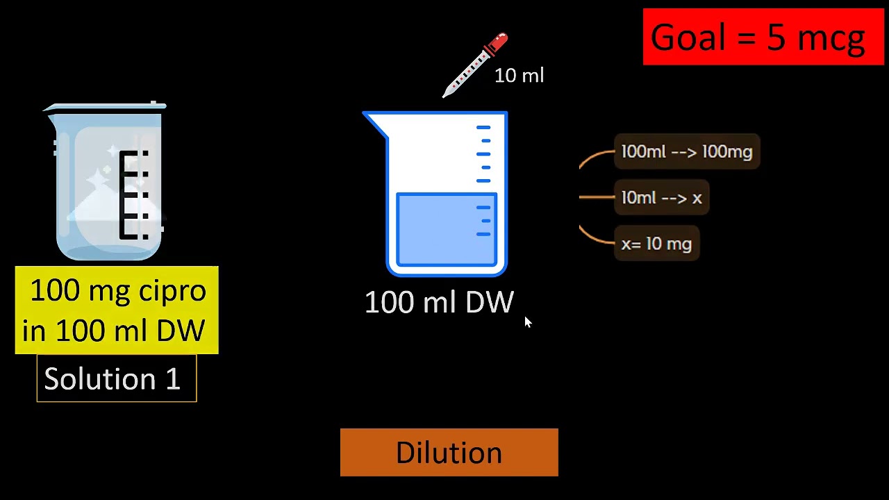
calibration curve - ciprofloxacin assay
2K
Linear regression derives the equation y = mx + b from calibration data. The slope (m) is calculated using two points: m = (Y2-Y1)/(X2-X1). The intercept (b) uses mean values: b = Ȳ - mX̄. These parameters enable prediction of unknown concentrations from measured absorption values. For example, with m=1 and b=-2, a measured absorption of 2.9 yields a predicted concentration of 4.9 micrograms.
Click to watch →

Analisis asam salisilat
444
The calibration curve is constructed by measuring absorbance of each standard at λmax (541 nm). The regression equation y = mx + b is generated, where y is absorbance, x is concentration, m is slope, and b is intercept. The correlation coefficient (R²) indicates fit quality, with values close to 1 indicating strong linear relationship. For example, y = 0.00494x - 0.0206 with R² = 0.998. This equation enables calculation of unknown sample concentrations from their absorbance values.
Click to watch →

Curvas de Calibración. Estándar externo
2.9K
The calibration curve follows a linear regression equation: Y = MX + B, where Y represents the measured signal, M is the slope (representing sensitivity), X is the analyte concentration, and B is the intercept. The intercept can be positive or negative depending on where the line crosses the Y-axis. This equation allows calculation of unknown concentrations from their measured signals.
Click to watch →
Deep Dive
Fundamental concepts of laboratory quality control, including the definitions of precision, accuracy, and experimental error.

Accuracy vs Precision.Systematic error vs Random error.Lab interview question.Easy definitions
333
This section establishes the foundational concepts of accuracy and precision in laboratory testing. Accuracy measures how close measured values are to the true target or accepted value, indicating reliability of results. Precision measures how close repeated measurements of the same sample are to each other, indicating consistency and repeatability. The instructor explains that accuracy focuses on closeness to the target while precision focuses on repeatability. Diagrams illustrate three scenarios: accurate but not precise (values near target but scattered), precise but not accurate (values clustered but away from target), and both accurate and precise (values clustered near target). Low accuracy indicates systematic error, while low precision indicates random error. These concepts form the basis for understanding laboratory quality control and interpreting QC graphs.
Click to watch →

CNU 2025 | Bloco 8 | Semana Decisiva - Controle de qualidade em laboratório
448
Precision (reprodutibilidade) refers to the ability of a method or equipment to produce consistent results when repeating analyses, regardless of whether those results are close to the true value. Accuracy (exatidão) refers to how close the results are to the true or target value. A method can be precise (results are close to each other) but not accurate (results are far from the true value). Internal quality control evaluates precision, while proficiency testing (external quality control) evaluates accuracy. The coefficient of variation (CV) is used to assess precision through variability between multiple analyses.
Click to watch →

Accuracy vs Precision | Types of Errors | Random error vs Systemic error | SD vs CV which is better
618
Accuracy measures how well a measurement agrees with the accepted or true value, indicating closeness to the true value. Precision measures how different measurements agree with each other, indicating the degree of fluctuation or repeatability. High precision means measurements are close to each other, while high accuracy means measurements are close to the true value. Precision detects random errors described by SD and CV, while accuracy detects systemic errors described by bias. Using a target diagram: measurements close to each other but far from target indicate high precision but poor accuracy; scattered measurements far from target indicate poor precision and accuracy.
Click to watch →

INTRODUCCIÓN AL CONTROL DE CALIDAD EN EL LABORATORIO CLÍNICO
30K
Precision is the degree of agreement between multiple results from the same sample measurement. Accuracy (veracidad) is the closeness between average measurements and the true value. Total error combines both precision and accuracy. A laboratory can have good precision but poor accuracy, which would not be acceptable. The total error is calculated as the sum of the coefficient of variation (precision) and the bias (accuracy). To determine if total error is acceptable, it must be compared against established acceptable total error limits for each analyte. Both internal and external quality control are necessary to obtain both precision and accuracy data.
Click to watch →

Quality Control of Clinical Laboratory
100
Accuracy is the closeness of a result to the actual value (true value), also called bias and representing systematic error. Precision (reproducibility/repeatability) is the closeness of values to each other when the same sample is tested repeatedly, representing random error dispersion. Both accuracy and precision are essential for reliable laboratory results. Four scenarios illustrate these concepts: (1) Accurate and precise - all results near the true value and close to each other, (2) Precise but not accurate - results close to each other but away from the true value (indicating systematic error), (3) Accurate but not precise - results near the true value but scattered (indicating reproducibility error), and (4) Neither accurate nor precise - results scattered and away from the true value.
Click to watch →
Prerequisite Knowledge
- Concept 01Understanding of the Beer-Lambert Law and the mathematical relationship between absorbance and solute concentration.
- Concept 02Basic statistical concepts, specifically how to calculate and interpret the mean, variance, and standard deviation of a dataset.
- Concept 03Familiarity with standard calibration curves and linear regression analysis (y = mx + c) in quantitative analysis.
- Concept 04Fundamental concepts of laboratory quality control, including the definitions of precision, accuracy, and experimental error.
Subsequent Learning
- Step 01Comprehensive study of ICH (International Council for Harmonisation) Q2(R1) guidelines for the validation of analytical procedures.
- Step 02Application of validation parameters in regulated environments, such as FDA, GMP, or ISO/IEC 17025 accredited laboratories.
- Step 03Advanced statistical tools for analytical chemistry, including ANOVA, F-tests, and t-tests for method comparison.
- Step 04Designing and executing robustness and ruggedness testing to evaluate the stability of an analytical method against minor deliberate variations.
Morning Mindset
Overcoming Negativity
Navigating Struggles
Self-Belief
Resilient Actions
Daily Growth
Morning Mindset
0:00Playing Section
- 1
Starts with a positive morning routine and goal-setting.
- 2
Emphasizes controlling steps and learning from mistakes.
- 3
Focuses on daily repetition to build success habits.
The Measurement Uncertainty (GUM) Paradigm vs. Classical Validation Metrics
While classical Quality Control (QC) method validation heavily relies on calculating discrete thresholds like the Limit of Detection (LOD) and Limit of Quantitation (LOQ) using standard deviations of blanks, metrologists increasingly advocate for the 'Uncertainty of Measurement' approach outlined in the ISO Guide to the Expression of Uncertainty in Measurement (GUM). Critics of traditional validation argue that traditional LOD and LOQ calculations are statistically arbitrary, highly dependent on sample matrix variations, and fail to account for the total uncertainty budget across the entire analytical range. Instead of treating detection as a binary threshold, the GUM framework quantifies a continuous interval of uncertainty for every measurement. This perspective suggests that traditional validation metrics oversimplify analytical performance, and that reporting a comprehensive measurement uncertainty budget provides a more transparent, scientifically rigorous, and internationally standardized representation of method reliability.
Deep Dive
Comprehensive study of ICH (International Council for Harmonisation) Q2(R1) guidelines for the validation of analytical procedures.

Joint US FDA – Health Canada ICH Public Meeting | D1S07-Q2(R2)/Q14, Revision of Q2(R1) Analytical...
278
The ICH Q2(R2) guideline revises the 1990s-era Q2(R1) to provide more flexible validation requirements for modern analytical technologies including multivariate spectroscopy, while Q14 introduces a systematic framework for analytical procedure development that integrates with the validation lifecycle, enabling pharmaceutical companies to develop, validate, and manage analytical procedures throughout the drug product lifecycle with greater scientific rigor and regulatory flexibility.
Click to watch →

ICH guidelines Quality
132.3K
ICH quality guidelines span 14 guidelines from Q1 to Q14. Q1 covers stability testing including Q1A (stability testing of new drug substances/products), Q1B (photo stability testing), Q1C (new dosage forms), Q1D (bracketing/matrixing designs), Q1E (stability data evaluation), and Q1F (stability data package for climate zones 3/4). Q2 focuses on analytical validation with Q2R1 covering analytical procedure validation and Q2R2 addressing analytical procedure development. Q3 addresses impurities including Q3A (drug substance impurities), Q3B (drug product impurities), Q3C (residual solvents), Q3D (elemental impurities), and Q3E (extractables/leachables control). These guidelines provide standardized frameworks for ensuring pharmaceutical product quality throughout development and manufacturing processes.
Click to watch →

ICH Q2 Validation of Analytical Procedures
629
The ICH Q2 guideline establishes comprehensive requirements for validating analytical procedures in pharmaceuticals, ensuring methods are reliable, precise, and accurate through systematic validation parameters including specificity, linearity, range, accuracy, precision, detection and quantitation limits, robustness, and system suitability, across stages of method development, initial validation, and ongoing verification to maintain consistent product quality and safety.
Click to watch →

Analytical method validation ICH Q2(R1) pharmaceutical || HPLC || GC || RS by HPLC || Assay - part-2
101
ICH Q2(R1) provides the unified guideline for analytical method validation in pharmaceutical industry, replacing the previous Q2A and Q2B guidelines, and covers four validation categories: Category 1 for preservative APIs, Category 2 for identification and quantitative tests, Category 3 for four conditions, and Category 4 for specific cases, with supporting chapters 1224 (analytical procedure transfer), 1225 (analytical procedure validation), and 1226 (analytical procedure verification) addressing method suitability and implementation.
Click to watch →
Accuracy Parameter in Analytical Method Validation | ICH Q2(R1)
305
Accuracy in analytical method validation, as per ICH Q2(R1) guidelines, is defined as the closeness of agreement between test results obtained by an analytical method and the true or accepted reference value, and is evaluated through recovery studies where samples are spiked with known amounts of analyte at 50%, 100%, and 150% concentration levels, with three replicates at each level; the percent recovery is calculated using the formula (amount recovered ÷ amount added) × 100, and acceptance criteria typically range from 98-102% for assay methods and 80-120% for impurity methods, with accuracy being essential for assay, impurity, and content uniformity methods but not required for limit tests.
Click to watch →
Deep Dive
Application of validation parameters in regulated environments, such as FDA, GMP, or ISO/IEC 17025 accredited laboratories.

Limites de Detecção e de Quantificação
25.1K
ISO/IEC 17025 requires laboratories to select methods meeting client requirements (Clause 4.4.1.C). Preference goes to internationally recognized methods (standards, pharmacopoeias, environmental standards) which don't require full validation. However, laboratories must confirm their capability to operate these methods through internal testing, demonstrating competence via detection limit and repeatability data. LOQ values must accompany method verification requests. This framework balances regulatory compliance with practical laboratory operations.
Click to watch →
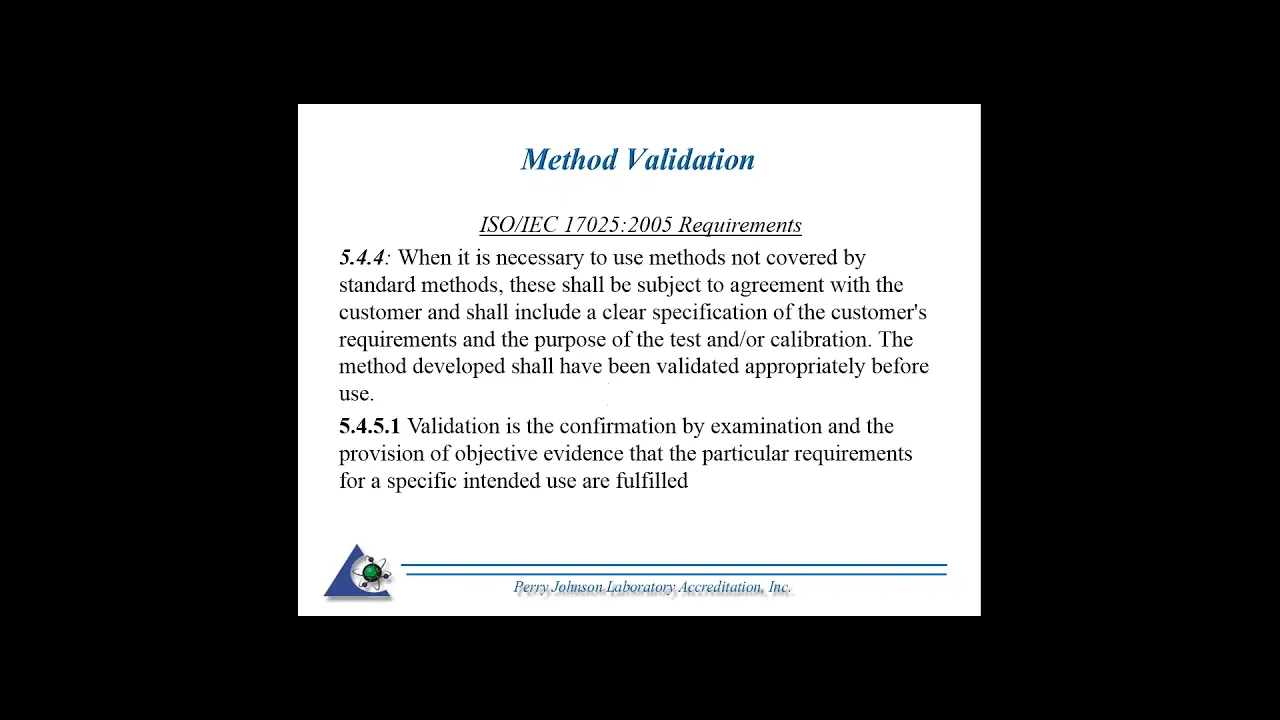
Method Validation in Accordance to 17025-How to meet the requirement of the standard
4K
Method validation under ISO/IEC 17025 requires laboratories to validate non-standard methods (including developed methods, modified standard methods, and amplifications) through appropriate techniques such as calibration with reference materials, comparison with other methods, interlaboratory comparisons, proficiency testing, systematic assessment of influencing factors, and uncertainty analysis; laboratories must document validation procedures and record whether the method is fit for its intended use, with the extent of validation depending on the degree of departure from standard specifications and the specific application requirements.
Click to watch →
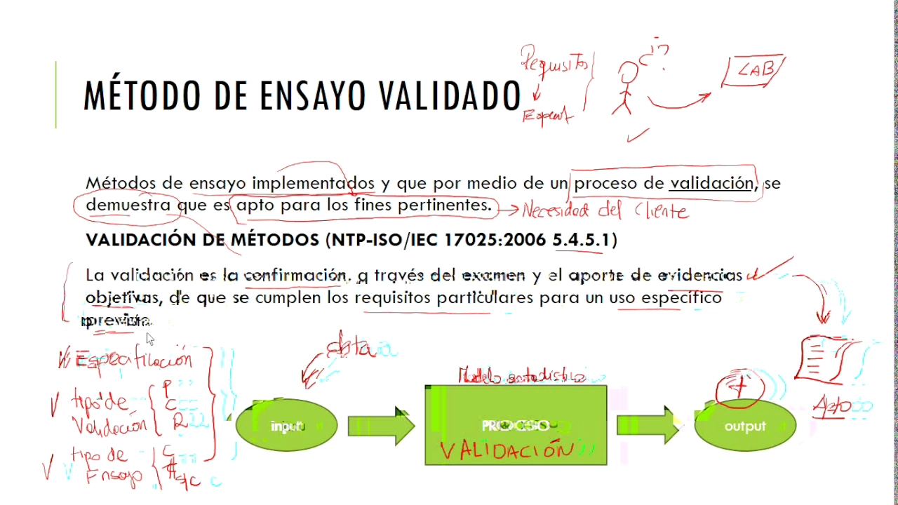
Performance de un método de ensayo validado (1/2) - Teoría
5K
Method validation is the process of demonstrating that an implemented test method meets requirements for its intended use, as defined in ISO 17025 clause 5.4.5.1. The process transforms inputs (client specifications, validation type, statistical models, method type) into outputs (objective evidence reports). ISO 17025 mandates validation for non-standardized methods, in-house methods, standardized methods used outside scope, and modified methods. Validation approaches differ by method type—qualitative methods don't require linearity validation, and volumetric/gravimetric methods don't use concentration-dependent calibration curves. ISO 17025 clause 5.4.5.3 specifies ten validation parameters: trueness, precision, selectivity/specificity, detection limit, quantification limit, linearity, working range, sensitivity, robustness, and uncertainty. Validation can be complete (all ten parameters) or partial (typically trueness and precision). ISO 17025:2014 provides three mechanisms for demonstrating accuracy: using certified reference materials (CRMs), fortification with known values using standard solutions, and comparison with validated methods. A fourth approach involves interlaboratory comparisons. CRMs are most expensive but most reliable, requiring multiple replicates and statistical tests. Standard solutions are less expensive but matrix-specific. Comparison with validated methods is most cost-effective but requires access to the validated method's equipment.
Click to watch →

ANAB Webinar: To Validate or Verify, that is the Question
668
This section establishes the foundational regulatory framework distinguishing verification from validation under ISO/IEC 17025. Verification provides objective evidence that established performance characteristics can be met in the laboratory, while validation determines and establishes those characteristics for unvalidated methods. Verification is mandated for equipment conformity checks (6.4.4) and standard method introduction (7.2.1.5). Validation is required for non-standard methods, laboratory-developed methods, and modified standard methods. Standard methods are those already validated and published through international, national, or peer-reviewed sources, requiring only verification. Non-standard methods require full validation as extensive as necessary. Computerized systems require adequacy verification through pre-use testing, periodic revalidation, or change-triggered revalidation.
Click to watch →

ISO/IEC 17025 | La selección, verificación y validación del método en un sistema de gestión ISO17025
14K
ISO/IEC 17025 requires laboratories to systematically select, verify, and validate methods through a six-step process: (1) Identify the laboratory's scope using requirement 5.3, (2) Classify methods as standardized, laboratory-developed, or modified, (3) Ensure adequate resources including personnel competence, infrastructure, equipment, and traceability, (4) Verify standardized methods by confirming they meet specifications, (5) Validate modified or laboratory-developed methods by demonstrating suitability for intended purpose, and (6) Continuously monitor method performance through internal quality control and inter-laboratory comparisons. Key performance characteristics to evaluate include measurement range, accuracy, uncertainty, detection limit, quantification limit, selectivity, linearity, repeatability, reproducibility, and resistance to matrix interference.
Click to watch →
Deep Dive
Advanced statistical tools for analytical chemistry, including ANOVA, F-tests, and t-tests for method comparison.

آموزش شیمی تجریه 1-فصل دوم: آمار و خطا | حل مسائل - قسمت اول
200
Three essential statistical tests for analytical chemistry: (1) F-test compares precision (repeatability) between methods - used when comparing variances, (2) T-test determines if there is a significant difference between means or detects systematic errors, (3) Q-test identifies outliers in data sets. The F-test is specifically used for comparing precision, which is what 'repeatability' refers to in analytical method comparison. These tests are commonly used in university exams and graduate entrance examinations.
Click to watch →

CHE1010 2024 EXAM SECTION C SOLVED
635
This section covers statistical methods for comparing analytical methods. First, calculate standard deviation using: S = √[Σ(xi - x̄)² / (n-1)], where xi are individual values, x̄ is the mean, and n is sample count. Second, use the F-test to compare variances between methods: F_calc = variance of method being tested / variance of established method. Third, calculate degrees of freedom: v1 = n1 - 1, v2 = n2 - 1. Fourth, find F_tabulated from F-table using degrees of freedom. Fifth, compare F_calc with F_tabulated: if F_calc < F_tabulated, no significant difference exists. This statistical approach validates analytical method reliability.
Click to watch →

Data Analytics In Excel Full Course | Data Analytics Course For Beginners | Intellipaat
7.6K
T-tests compare group means: one-sample (single group vs value), paired (related samples), and two-sample (independent samples). Assumptions include random sampling, normality, and homogeneity of variances. The f-test checks variance equality using f-distribution. ANOVA extends comparison to three+ groups: one-way (single factor with ≥3 categories) and two-way (two factors with replication or without).
Click to watch →

Examination Based Last hours preparation for Job Holder Students
651
T-test for single mean: t = (x̄-μ)/(s/√n). T-test for double mean: t = (x̄1-x̄2)/√(s1²/n1 + s2²/n2). For paired samples: t = d̄/(s/√n). T-test for correlation coefficient: t = r√(n-2)/√(1-r²). F-test for variance ratio: F = s1²/s2² (larger variance over smaller). ANOVA involves SST, SSR, and SSC with F = MSR/MSC. Chi-square for Goodness of Fit: χ² = Σ(O-E)²/E. Chi-square for Independence: χ² = Σ(O-E)²/E with E = (row total × column total)/grand total.
Click to watch →

TUTORIAL OUTLIERS, SIGNIFIKANSI (UJI T) DAN INSTALL ORANGE DATA MINING
477
This section advances students' statistical capabilities by introducing variance comparison and multi-group analysis. The instructor explains that F-tests compare variances between two groups, available only as two-tailed tests in Excel. Students learn to access F-tests through Data Analysis and understand the distinction from T-tests which compare means. The section then transitions to ANOVA (Analysis of Variance), explaining its purpose for comparing three or more group means simultaneously. Students learn to access ANOVA through Data Analysis, configure input ranges, and interpret output tables containing degrees of freedom, sum of squares, mean squares, F-statistics, and p-values for determining significant differences across multiple groups.
Click to watch →
Deep Dive
Designing and executing robustness and ruggedness testing to evaluate the stability of an analytical method against minor deliberate variations.
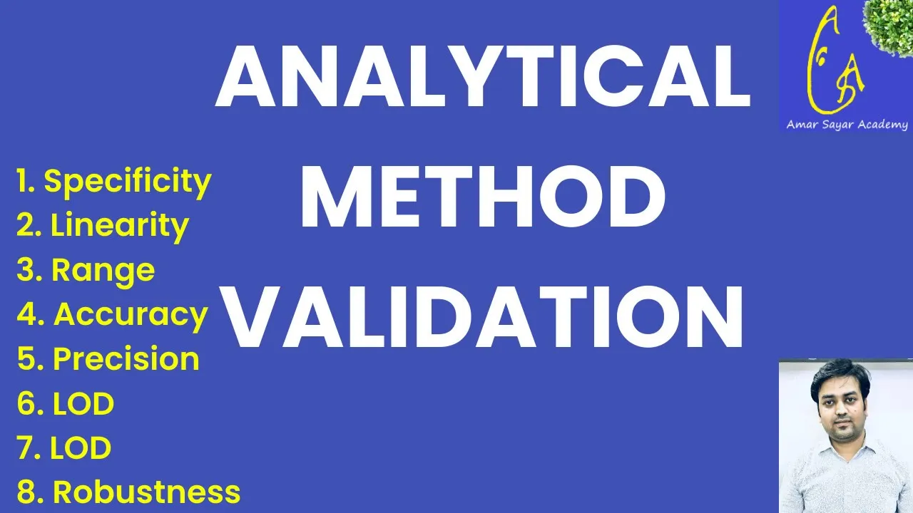
VALIDATION OF ANALYTICAL METHOD | Method validation | Validation of an analytical procedure
130K
Robustness is the ability of an analytical procedure to remain unaffected by small but deliberate variations in method parameters. These variations may include pH, mobile phase composition, flow rate, temperature, and other experimental factors. Robustness testing ensures that the method produces reliable results even when minor changes occur in the experimental conditions.
Click to watch →

Quality Control Practical || Titration & Problems
598
Robustness is assessed by making small changes to the method (such as mobile phase composition) and comparing results. Ruggedness is assessed by making significant changes (such as changing the analyst, laboratory, or time of analysis). For both, calculate recovery percentages for the new conditions, then calculate RSD: RSD% = (Standard Deviation / Mean Recovery) × 100. If RSD is less than 2%, the method is considered robust or rugged.
Click to watch →

Validasi Metode Analisis Part 1
4.4K
Robustness evaluates method stability under small deliberate variations in parameters like pH, flow rate, or temperature. Ruggedness tests method performance under more extreme variations including different laboratories, analysts, and instruments. A method passing ruggedness testing may be suitable for pharmacopeial inclusion, allowing industries to verify rather than validate methods. Revalidation is required when validation parameters fall outside acceptance criteria, when significant procedure changes occur, or when pharmaceutical formulations change. This ensures methods remain suitable for their intended purpose after modifications, particularly important for multi-ingredient pharmaceutical products where changes to one component may affect the entire analytical method.
Click to watch →
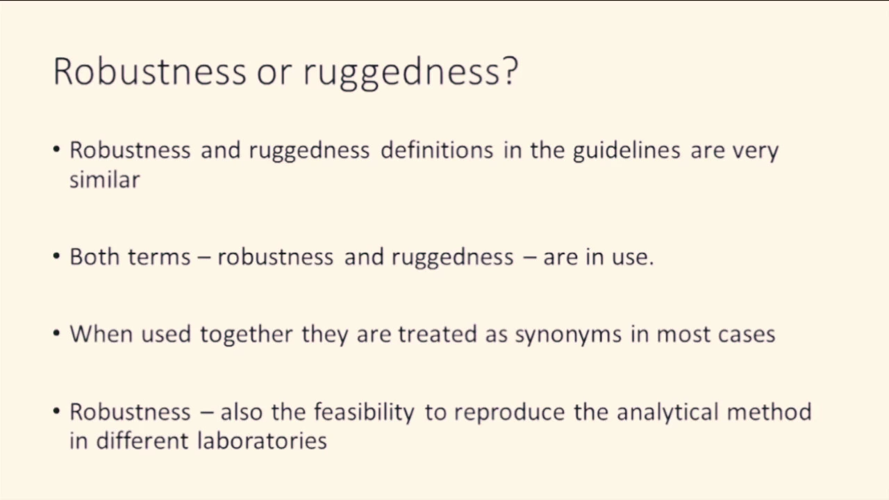
Robustness and ruggedness introduction
7K
Robustness and ruggedness are analytical method validation parameters that assess a method's ability to remain unaffected by small variations in method parameters (such as mobile phase composition, column temperature, and injection volume) and environmental factors (like room temperature and humidity), ensuring reliable results during normal usage; robustness typically refers to stability against intrinsic method variations within the same laboratory, while ruggedness addresses reproducibility across different laboratories and conditions.
Click to watch →

Validação de Métodos Analíticos: ROBUSTEZ
600
Robustness is a validation parameter that measures an analytical method's ability to withstand small, deliberate variations in experimental conditions without producing significant changes in results; it is evaluated by intentionally modifying individual method parameters (such as wavelength, pH, mobile phase composition, extraction time, or solvent purity) and comparing the modified results to the original method using statistical analysis to ensure the method remains reliable under minor variations.
Click to watch →
Morning Mindset
Overcoming Negativity
Navigating Struggles
Self-Belief
Resilient Actions
Daily Growth
Morning Mindset
0:00- 1
Starts with a positive morning routine and goal-setting.
- 2
Emphasizes controlling steps and learning from mistakes.
- 3
Focuses on daily repetition to build success habits.
The Measurement Uncertainty (GUM) Paradigm vs. Classical Validation Metrics
While classical Quality Control (QC) method validation heavily relies on calculating discrete thresholds like the Limit of Detection (LOD) and Limit of Quantitation (LOQ) using standard deviations of blanks, metrologists increasingly advocate for the 'Uncertainty of Measurement' approach outlined in the ISO Guide to the Expression of Uncertainty in Measurement (GUM). Critics of traditional validation argue that traditional LOD and LOQ calculations are statistically arbitrary, highly dependent on sample matrix variations, and fail to account for the total uncertainty budget across the entire analytical range. Instead of treating detection as a binary threshold, the GUM framework quantifies a continuous interval of uncertainty for every measurement. This perspective suggests that traditional validation metrics oversimplify analytical performance, and that reporting a comprehensive measurement uncertainty budget provides a more transparent, scientifically rigorous, and internationally standardized representation of method reliability.
Understanding of the Beer-Lambert Law and the mathematical relationship between absorbance and solute concentration.
Basic statistical concepts, specifically how to calculate and interpret the mean, variance, and standard deviation of a dataset.
Familiarity with standard calibration curves and linear regression analysis (y = mx + c) in quantitative analysis.
Fundamental concepts of laboratory quality control, including the definitions of precision, accuracy, and experimental error.
Comprehensive study of ICH (International Council for Harmonisation) Q2(R1) guidelines for the validation of analytical procedures.
Application of validation parameters in regulated environments, such as FDA, GMP, or ISO/IEC 17025 accredited laboratories.
Advanced statistical tools for analytical chemistry, including ANOVA, F-tests, and t-tests for method comparison.
Designing and executing robustness and ruggedness testing to evaluate the stability of an analytical method against minor deliberate variations.
64K views762likes12:22@chemist_isiOriginal Release: 2018-01-21
step one wake up brother gonna rise to the sun step two get some good some food in your step three they grow hard about what you want to be step four everybody just do your thing wake up today's gonna be a good day wake up today's [Music] gonna be a good day today's [Music] gonna be a good day wake up today's gonna be a good day set your affirmations aspirations I got to do the aftermath of preparation [Music] one step at a time yeah that's how you make it set a goal you control and the steps you take them I'll try to pick one thought I have some concentration and if I make a mistake it's called education I try to do this every day call it replication wake up today's [Music] wake up wake up wake up today's gonna be a good day wake up today's gonna be a good day [Music] ups and downs just like every different season y'all sometimes I'm not other times I'm barely breathing though I always Gotta Fight Night from the demons yeah negative thoughts [Music] they'll never stop unless I can swap all the bad for the good in my head when I'm lost yeah so I'm a fake it till I make it positive thoughts are overtaking I got patience one day at a time it's how you operate a great flow you grow you show yourself the foundation stay away from all the that causes Temptation I know that I like to do it cause the sensation I live my life in my head like a narration don't expect greatness do my best man I'll take it wake up today's gonna be a good day wake up [Music] today's [Music] gonna be a good day [Music] [Music] accepted [Music] [Music] friends [Music] thank you [Music] foreign [Music] [Music] [Music] [Music] [Music] thank you [Music] thank you [Music] foreign [Music] thank you [Music] foreign [Music] thank you [Music] thank you foreign [Music] [Music] foreign [Music] thank you [Music] foreign [Music] thank you [Music] foreign [Music] foreign [Music] foreign [Music] [Music] foreign [Music] [Music] [Music]
Up Next

3:46
Egyptian Blue: Ancient Pigment's Modern Applications in Forensics and Medicine
@SciShow
284.8K views•2018-01-04

83:56
Biocatalysis and Catalysis in Islatravir Synthesis | Merck Webinar
@SCIwheresciencemeetsbusiness
675 views•2020-10-08
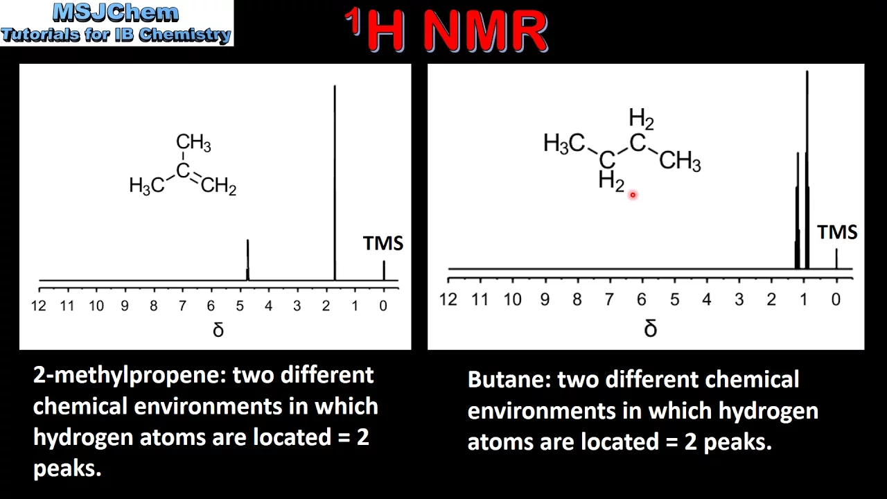
10:06
1H NMR: Determining Number of Peaks from Structure
@MSJChem
59.2K views•2017-04-06

17:31
Edible Water Bottles: A DIY Guide to Sodium Alginate Spherification
@ryan
10.5M views•2019-06-21
Related Study Plans & Knowledge Roadmaps
Structured learning paths in Chemistry
chemistry
Nuclear Chemistry: Decay, Meds & Fuel Cycle
01Introduction to Nuclear Structure and Radioactivity
02Decay Dynamics and Kinetics
03Radiation Interaction and Detection
+ 2 more learning modules
24h5 modules
Explore Roadmap
chemistry
Supramolecular Chemistry: Forces & Machines
01Foundations of Chemical Bonding and Intermolecular Forces
02Introduction to Host-Guest Chemistry
03Thermodynamics and Dynamics of Self-Assembly
+ 2 more learning modules
16h5 modules
Explore Roadmap
chemistry
Photochemistry: Excited States & Reactions
01Foundations of Light-Matter Interactions
02Molecular Orbitals and Electronic States
03Photophysical Processes and Jablonski Diagrams
+ 2 more learning modules
18h5 modules
Explore Roadmap
chemistry
Coordination Chemistry: Bonding & Properties
01Introduction to Transition Metals and Ligands
02Crystal Field Theory (CFT) and Geometry
03Magnetic Behavior and Spin States
+ 2 more learning modules
14h5 modules
Explore Roadmap