







![[Math 23] Lec 4.2 Fundamental Theorem of Line Integrals and Independence of Path](https://i.ytimg.com/vi_webp/E1BVK8bd0yk/maxresdefault.webp)


![CAL III [Final] day 3 ] | พี่ติวน้อง โยธาจุฬาฯ 1/2568](https://i.ytimg.com/vi_webp/dS4hQsQ7-ws/maxresdefault.webp)





![[직장인과 문과생을 위한 수학교실 4기] 27. 미적분학의 기본정리 2변수 함수로 확장하기](https://i.ytimg.com/vi/dXJCt4Hw-_k/maxresdefault.jpg)





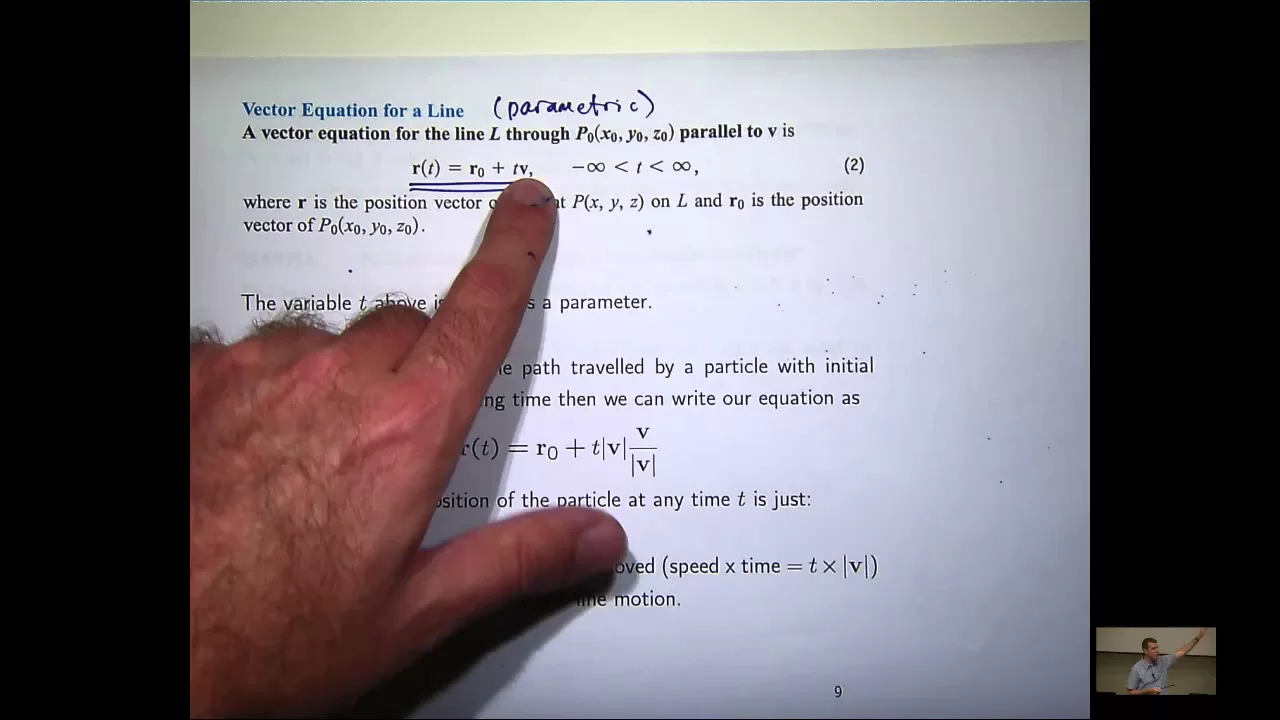
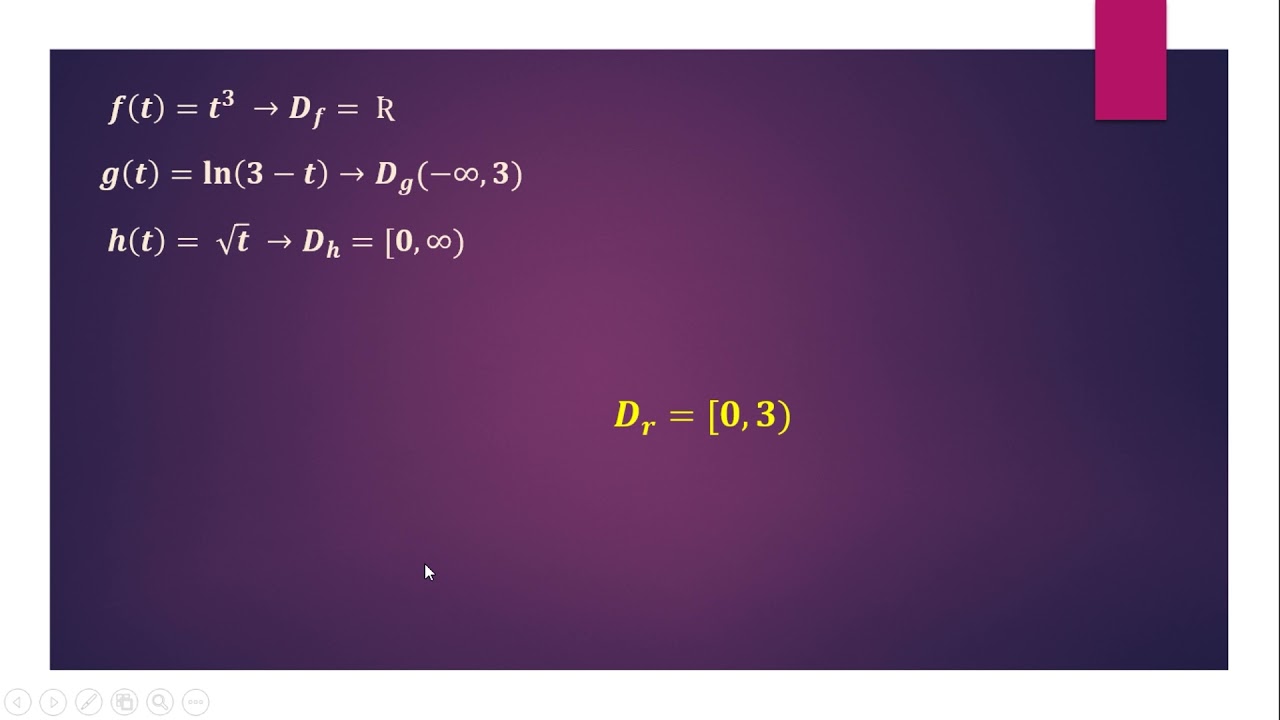
Line integrals extend the concept of 1D integration to higher dimensions by integrating a function along a curve rather than along a straight line. The process involves parameterizing the curve using a vector-valued function r(t), then calculating the integral as ∫f(r(t))||r'(t)||dt, where ||r'(t)|| represents the magnitude of the derivative (the infinitesimal step ds along the curve). This approach transforms the abstract concept of integrating along a curve into a concrete calculation using standard integration techniques, with the choice of parameterization significantly affecting computational complexity.
Line Integrals Explained: Intuitive Multivariable Calculus Tutorial
Added:Understanding of single-variable integration, specifically the concept of Riemann sums and calculating definite integrals.
Familiarity with parametric equations and vector-valued functions to represent curves in 2D and 3D space.
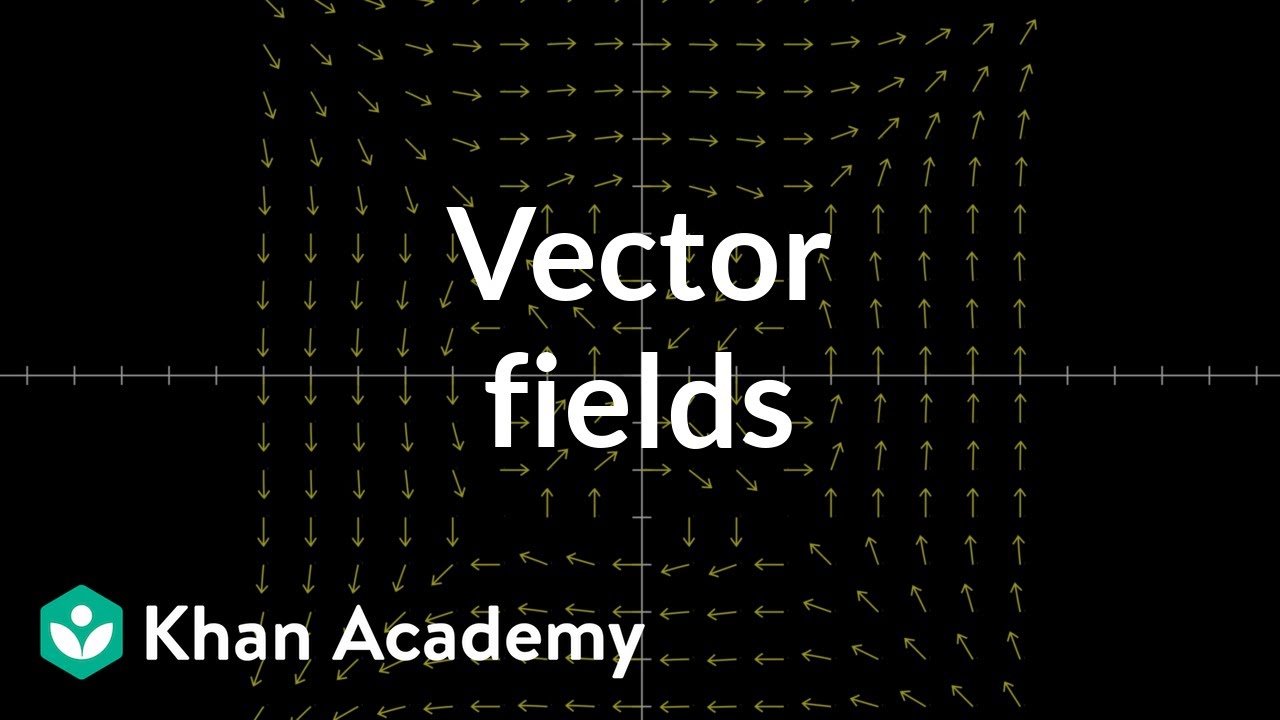
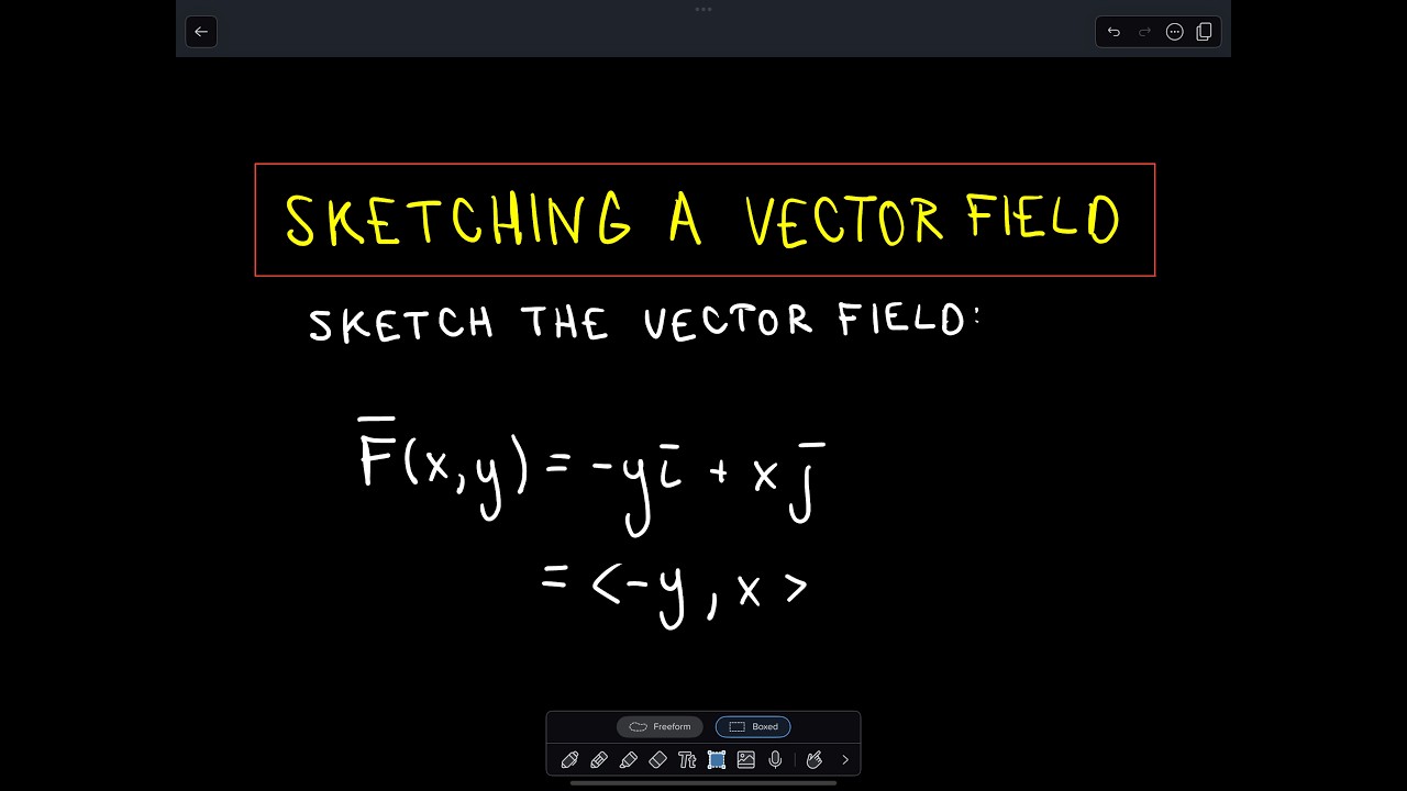
Basic knowledge of vector fields, including how to represent and evaluate vectors at different points in space.
An understanding of partial derivatives and the gradient vector of a multivariable function.
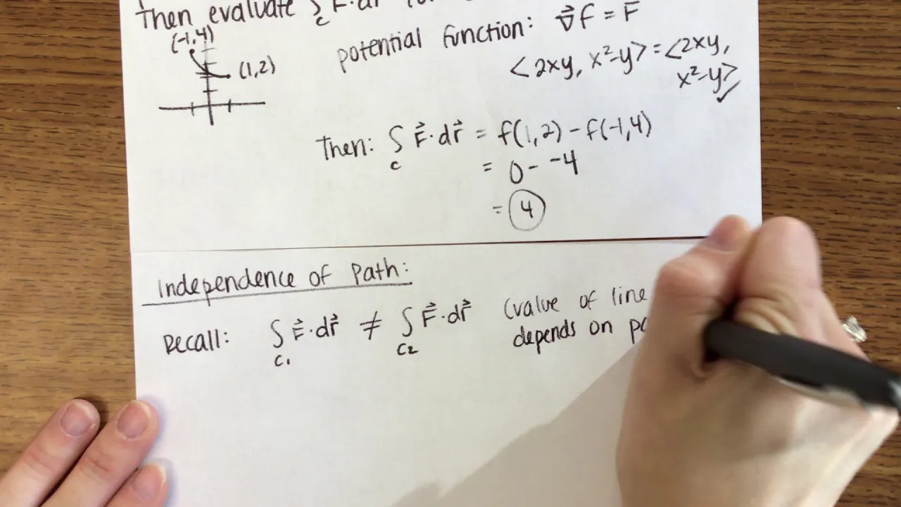
The Fundamental Theorem of Line Integrals and the concept of path independence in conservative vector fields.
Green's Theorem, which connects a line integral around a simple closed curve to a double integral over the plane region it bounds.
Surface integrals of scalar and vector fields, extending integration from 1D curves to 2D surfaces in 3D space.
Stokes' Theorem and the Divergence Theorem, representing high-dimensional generalizations of the Fundamental Theorem of Calculus.
Physical applications in engineering and physics, such as calculating mechanical work, fluid circulation, and analyzing electromagnetic fields.
262.3K views11Klikes21:02Original Release: 2024-08-19
when I was in sixth [Music] grade I learned about functions for the first time like this one y = 2x you put in one thing and it gives you back two nice and then I went to high school and took pre-calculus and that class went something like this you guys like f ofx = X2 right now what if I make it FX = x^2 + y^2 domain [Music] expansion multivariable and now you can graph cylinders and spheres and surfaces and planes and heles all using mathematical equations in 3D okay maybe it wasn't that epic but that idea the expansion of old Concepts into new domains is a key Cornerstone of mathematics and it's applicable to so many different areas including calculus and integration and today that's EX exactly what I'm going to do take the idea of an ordinary 1D integral and expand it to higher Dimensions to describe line integrals I had promised in a previous video I would give a more detailed explanation of these and so here it is going into this video I'm going to assume that you have a basic understanding of how integration is done in 1D calculus I'm also going to assume you're somewhat familiar with the concept of an input space Vector valued functions and parameterization of Curves if you're not I would suggest watching my previous video on this topic in this video I'll be talking solely about the basics of line integrals where they come from the intuition behind them and how to calculate them for ordinary functions I won't be talking about line integrals over Vector Fields that's a topic I'm going to say for a different video since there's significantly more depth and Nuance to go into so let's get into it to talk about line integrals let's first start in single variable or 1D calculus with ordinary 1D integrals we'll see that line integrals are actually a pretty simple extension of regular integration into higher Dimensions I mean that's really what multivariable calculus is all about recall that 1D calculus is called 1D because we're working with functions with only one input variable denoted X meaning that our input space is onedimensional we always have one output variable denoted y this means we can graph our functions input and output in 2D let's use a relatively simple example the function Square < TK of X the traditional concept of a 1D integral involves taking the area under this curve and that's definitely true but let's look at it through a different lens let's bring ourselves down to one dimension the X dimension this right here is our input space the input space is a set of all possible values for our input which for us is just the real numbers if this term is unfamiliar to you check out my previous video on vectors and Vector fields or I Define it in irrelevant context so back to our 1D input space here X increases as we move to the right and decreases as we move to the left at each point on this x line there's an Associated yv value or output value I'm just labeling the output value corresponding to each input Point great now let's start the process of integrating we write our integral in this form integral of f ofx DX between some bounds of X let's pick one and 9 for our bounds for the sake of demonstration this DX tells us to take an infinite tmal step in the X Direction and since we're going from an initial value of one to a final value of 9 we'll move in the positive POS X Direction note that this is one of the two possible directions in our 1D input space we can either move to the right along this horizontal line or to the left and here we choose to move to the right we multiply the width of this infinitesimal step by the output value assigned to our starting point which here is a sare root of one which is just one since our DX is infinite asly small the output value at our starting point and our next point x = 1 + DX are pretty much the same we keep doing this over the entire length of the x-axis that we specified from x = 1 to xal 9 and add up each little product of DX and F ofx that's our total integral which is a single scaler value that's precisely what the symbols mean as well summing up all the products of F ofx and DX from x = 1 to xal 9 okay that's great but how about in higher Dimensions well I'm glad you asked let's move to three dimensions using the example function f ofx y = x^2 + y^2 domain expansion you can see the output of this function extending in and out of the page in the Z Direction now let's look only at the input space of this function which is the 2D XY plane and think about taking an integral remember with a 1D input space we could only move in two directions increasing X or decreasing X now that our input space is 2D we have a lot more directions we can move in infinitely many in fact and we don't even have to move in a straight line we can move in Squigly lines or Curves too so we need to ask a slightly different question what is the integral of our function f ofx comma y as we move along this curve or this one or this one now how do we write such an integral mathematically for a 2d input space we would write this as the integral of f ofx comma y d s over a curve C here the curve C is a line we're integrating over F of XY is the output of our 3D function and DS is an infinitesimally small movement along c the only difference between this an an ordinary integral in 1D calculus is that in 1D calculus your curve C was actually just the xais and therefore your DS was just DX this idea of taking an integral over a line may seem abstract but remember we did the exact same thing in 1D calculus let me demonstrate intuitively how it's done let's say we want to calculate the integral of our function f ofx y = + y^2 over a line segment going from 1A 1 to 3A 3 here's how that integral is calculated we'll start at 1 comma 1 find the output of our function at this point which is just two we then multiply that by an infinitesimally small piece of our line segment which we'll call DS which moves us to a new point on our line segment at this new Point we'd find the output of our function and again multiply it by DS we continue this for every point on the line segment adding up all those products of the function outputs and infin asmal steps along the integrating line to get the final value of the integral in this case that just so happens to come out to 52 < tk2 over 3 now an appropriate follow-up question would be how do we actually get to that number and the answer isn't obvious our DS is dependent on both the X and Y coordinates so it gets a little bit more complicated to describe what an infinite tmal step DS actually looks like mathematically but before I go there I want to address a question that may be lingering in some of your curious minds with 1D input spaces in other words an ordinary 1D calculus we could only take an integral over a line which was the x-axis with 2D input spaces we can take integrals over any line or curve existing in 2D space but can we not also take integrals over 2D surfaces now lines are 1D shapes and surfaces are 2D shapes so now that we have a 2d input space can we take integrals over 2D surfaces and the answer is yes we can that's how surface integrals work to get there we'd have to start talking about multi-dimensional integrals in other words integrals in more than one direction at the same time this is different from making our functions themselves multi-dimensional so I won't be talking about surface integrals in this video I just wanted to point this Nuance out to demonstrate what a line integral really is line integrals are 1D integrals they're integrals you take moving in One Direction along a 1D shape which is line and they end up producing a areas this contrasts with surface integrals which are 2D integrals integrals you take moving along two different directions over a 2d shape which is a Surface 2D integrals generate volumes there's a figure online that I really like which shows what line integrals really look like here it is they can still be thought of as areas just now these areas are along a squiggly path that can exist in three dimensions okay now that we've cleared up that Nuance let's go back and actually try to calculate these line integrals or at the very least turn this abstract mathematical expression into an expression that contains tangible numbers the problem here is this DS and this c what does it look like to integrate over a curve C or to take a step DS what exactly is DS how do we express it in terms of X and Y let's answer all those questions now our goal is going to be to express DS in terms of some differential that we have tangible bounds for so our first step is going to be to convert this DS into X and Y coordinates because we know how to work with those let's look at a general case first where we have some random undefined curve C and some given function f ofx comma Y where again in a 2d input space DS as we defined it previously is an infinitesimal step along our integrating curve C we can think of this infinite tmal step as a step in the direction tangent to the curve C at a given point and now this tangent step can be expressed in terms of infinitesimal steps in the X and Y directions DX is the X component of DS and Dy is the Y component from this drawing we can now see that DS can be simply found using the Pythagorean theorem DS s = dx2 + D y^2 so DS is the S < TK of dx2 + D y^2 let's substitute this into our original equation okay that's a step forward we've gotten rid of DS and put it in terms of DX and Dy but now this doesn't look like a traditional integral we've got two differentials in one integral and the differentials are in a square root it's a whole mess on top of that we still don't have proper bounds for our integral luckily there's a way we can fix this parameterization of the curve c what does that mean well this curve here can be written a some function of x y = f ofx we know that any function written like this can be Rewritten as two functions where Y and X are both a function of some new variable T which we call a parameter for example if you have the function y = 4x^2 you can rewrite that as y = t ^2 and x = t/ 2 so that when you substitute X of T into y of T you get the original function let's say that we can generally parameterize any curve including our integrating curve C from a single function y of X into two functions y of T and X of t x of T describes the X component of our curve While y of T describes the Y component both conveniently written as a function of T this also means we have bounds for our curve going from T KN which would output the starting point of our curve to T final which outputs the final point on our curve so how does parameterization help us well this is where things get a little hand wavy so stick with me here let's take our integral and throw in a DT over DT not changing anything just multiplying and dividing by a differential now let's move the DT in the denominator inside the square root when we distribute it out what we see is that we're left with two derivatives inside the square root dydt and dxdt which we can write also as y Prime of T and X Prime of T since we have functions y of T and X of T we can compute these derivatives rather easily and now we've practically solved our problem all that's left to do is to rewrite our function f of XY in terms of T add in the bounds we defined for our curve and bam we're done we have a tangible differential DT that gives us scalar bounds to integrate over and everything inside the integral is defined in terms of T awesome but we can take this formula a step further what if we want to take the line integral of a 4D function in other words one with a 3D input space well all we need to do is adjust this DS term by adding in a third input variable DZ DT and what if we're working in a 4D input space well then we a fourth input variable now you can see how this equation would get quite long if you have a very high dimensional space and also inconveniently it changes if we're dealing with different size input spaces so now the question is how can we generalize this well let's step back to a previous video where I said the following vvfs are equivalent to parametric representations of functions and that's the answer to ize this we can use Vector valued functions as a reminder Vector valued functions output a set of vectors that point from the origin to points on a curve to construct them you can just take the parameterization of a curve that you already have and throw on an I have Vector to the x of T term and a Jad Vector to the Y of T term this entire Vector value function called R of T describes describes our parameterized integrating curve in any number of Dimensions that it may exist so how do we describe this clunky square root in terms of R of T well with a bit of math we can see that this is just the magnitude or Norm of our derivative of our Vector valued function or vvf remember that Vector magnitudes can be calculated by simply applying a sort of Pythagorean theorem to the vector squaring each component adding them all up and then taking the square root therefore by taking the derivative of our vvf and then taking the magnitude of that derivative we end up with the square root term that was DS in our integral nice so we can simply substitute this vvf derivative magnitude for our square root component and then also substitute X of T and Y of t for just R of T and Bam we've got our line integral formula written in a tangible way that is generalizable to any number of Dimensions all thanks to Vector valued functions now let's see what this all looks like in an example let's use the example I was talking about earlier the line integral of the function f ofx y = X2 + y^ 2 over a straight line segment going from 1A 1 to 3A 3 we'll start by defining our integrating curve in terms of a parameter T luckily our integrating curve is really simple here it's just yal X so we can parameterize it as yal T and xal T so our Vector value function for this curve is just R of tal T IAT plus T jat this means our bounds are pretty simple as well going from 1A 1 to 3A 3 would be going from T = 1 to T = 3 now let's find the vector Norm of the derivative of R vvf the derivative is just IAT plus jat since both terms have a derivative of one and so the norm of the derivative is just squ < TK of 2 now let's look at our original function x^2 + y^2 and write it in terms of T well since both X and Y are equal to T that just makes our function 2 t^2 now throwing on our bounds we can see that we're left with a pretty simple integral which we can evaluate analytically like so and we find that the result is 52 < tk2 over 3 the same value I presented earlier for this line integral as a side note the example I chose here happened to be a very simple one because the derivatives of our vvf were constants you can imagine that for an integrating curve that's slightly more complicated this line integral can get very nasty to evaluate analytically and sometimes even impossible to evaluate at all for example if your integrating curve is something like X cubed we can parameterize it pretty simply as x = t and yal t cubed however now the norm of our R Prime of T term contains an x to the 4th term inside of a square root and inside the integral this square root term is multiplied by another term this makes this integral very difficult to evaluate analytically and sometimes impossible ultimately that means choosing your parameterization efficiently can be very important because some parameterizations will make the integration much easier than others and that's pretty much all I've got to say about line integrals of ordinary functions in the next video we'll talk about taking line integrals over Vector fields and we'll see why that is so important to the study of multivariable calculus thanks for watching and I'll see you in the next one [Music]
Up Next

21:36
Sequences and Their Limits: Quantifiers, Convergence, Proofs
@paulbamberg4017
106 views•2017-06-30

4:43
Elliptic Curve Cryptography Explained: ECC, ECDSA, ECDH
@PracticalNetworking
28.5K views•2024-10-21

10:44
Fourier Series Introduction: The Big Idea Explained
@DrTrefor
387K views•2021-05-03

6:00
The Mathematical Impossibility of Accurate World Maps
@Vox
23.3M views•2016-12-02
Related Study Plans & Knowledge Roadmaps
Structured learning paths in Mathematics
mathematics
Tensor Calculus: Vectors to Riemann Curvature
01Mathematical Foundations: Linear Algebra & Calculus
02Covectors, Dual Spaces, and Tensor Basics
03The Metric Tensor and Index Gymnastics
+ 2 more learning modules
40h5 modules
Explore Roadmap
mathematics
Gödel's Incompleteness: Logic, Proofs & Limits
01Introduction to Formal Systems & Hilbert's Dream
02Set Theory, Cardinality, and Cantor's Diagonal Argument
03Arithmetization and Gödel Numbering
+ 2 more learning modules
14h5 modules
Explore Roadmap
mathematics
Galois Theory: Fields, Groups & Solvability
01Foundations of Abstract Algebra: Groups & Fields
02Polynomials & Field Extensions
03Splitting Fields & Symmetries
+ 2 more learning modules
24h5 modules
Explore Roadmap
mathematics
Non-Euclidean Geometry: Models & Geodesics
01Euclid's Fifth Postulate and the Birth of New Geometries
02Hyperbolic Space and the Poincaré Disk Model
03Geodesics: Defining Straight Lines in Curved Spaces
+ 2 more learning modules
15h5 modules
Explore Roadmap