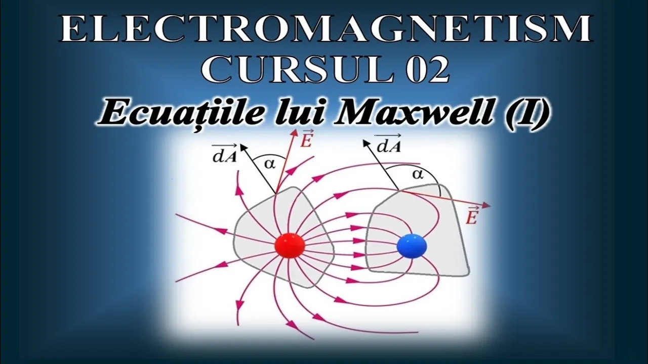


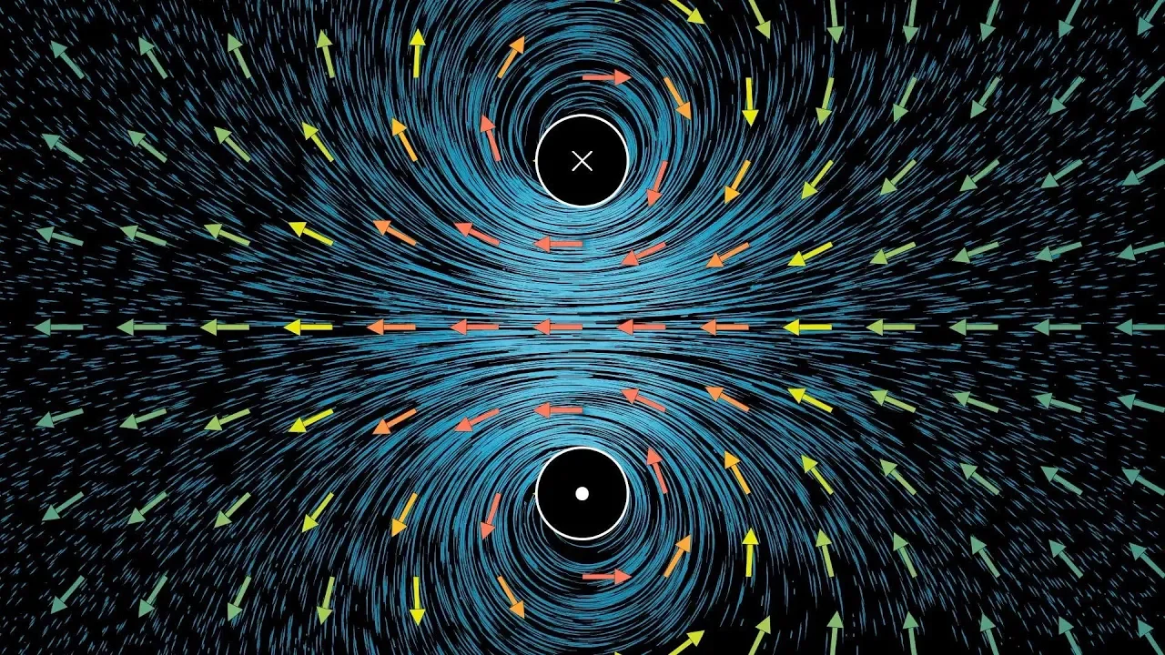
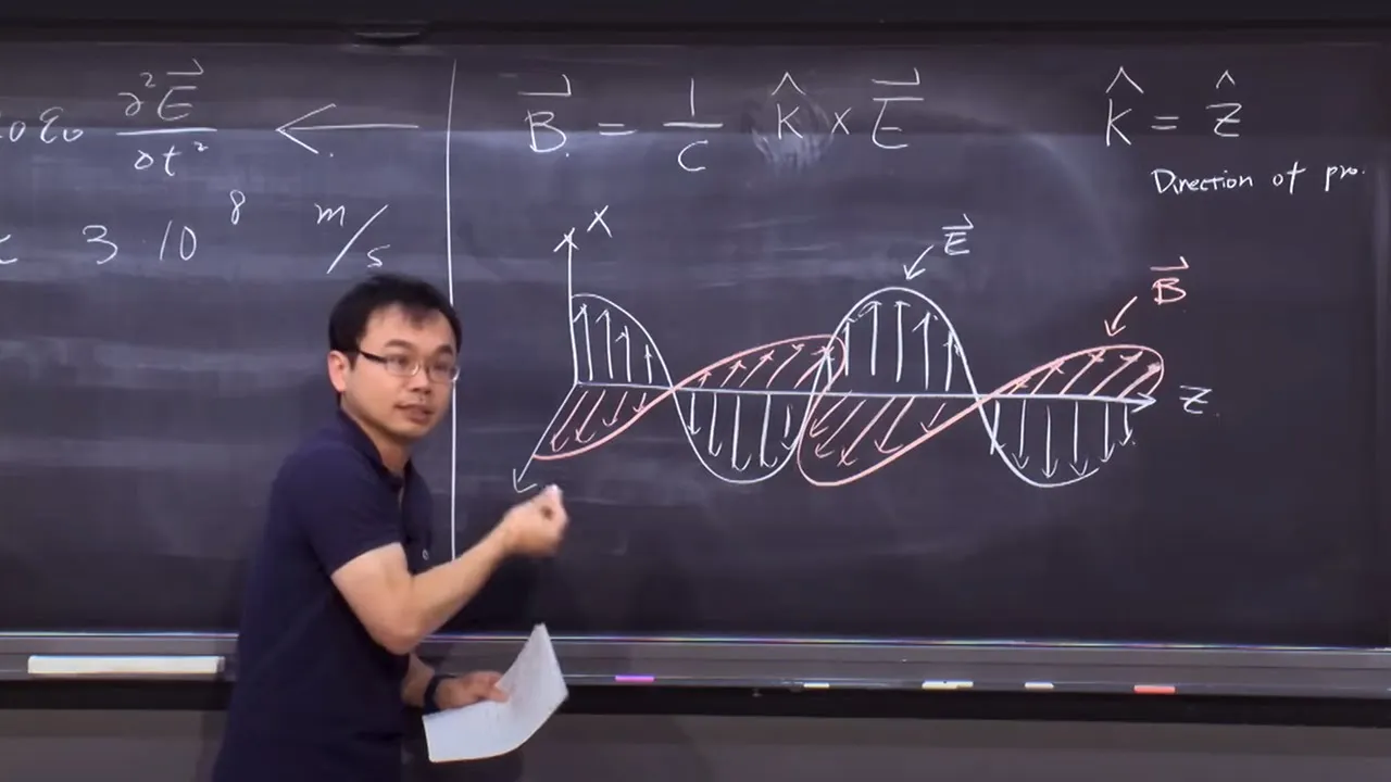


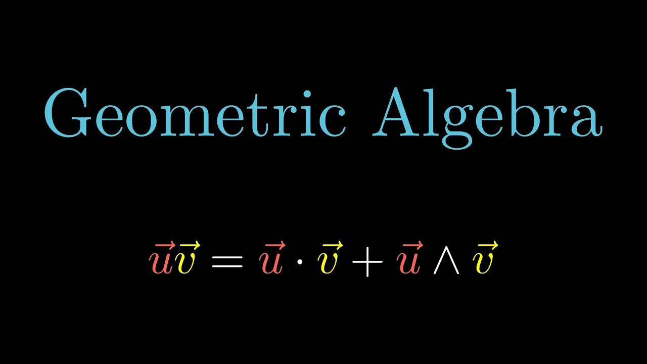








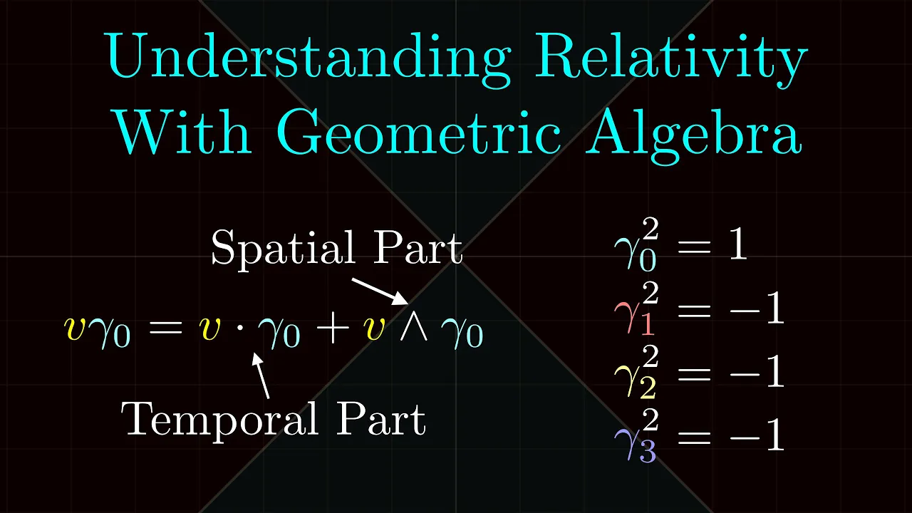









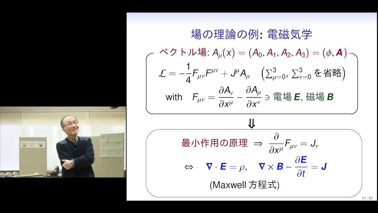


In geometric algebra, Maxwell's four vector equations can be unified into a single elegant equation using the geometric derivative operator (∂) acting on the electromagnetic field bivector F, expressed as ∂F = J, where J represents the current density; this approach naturally incorporates the vector nature of the electric field and the bivector nature of the magnetic field, allowing all four Maxwell's equations to emerge from one compact expression through the algebraic decomposition of the geometric derivative.
Deriving Maxwell's Equations in Geometric Algebra (QED Prereqs) 11
Added:Standard formulation of Maxwell's Equations using vector calculus, including concepts of divergence, curl, electric and magnetic fields.
Foundations of Geometric Algebra (Clifford Algebra), specifically the definitions of the geometric product, outer (wedge) product, and multivectors.
Basic special relativity, including the concept of four-vectors, Minkowski spacetime, and the Lorentz transformation.
The definition of the vector derivative (Dirac operator or del operator) in multidimensional spaces.
Formulating the Dirac Equation using Spacetime Algebra (STA) to describe relativistic spin-1/2 particles.
Applying Geometric Algebra to Quantum Electrodynamics (QED) for simplified gauge field calculations.
Analyzing the electromagnetic field tensor as a single bivector and exploring its Lorentz transformation properties.
Generalizing the formulation to non-Abelian gauge theories, such as Yang-Mills theory, using multivector calculus.
2.6K views115likes1:13:35Original Release: 2024-09-08
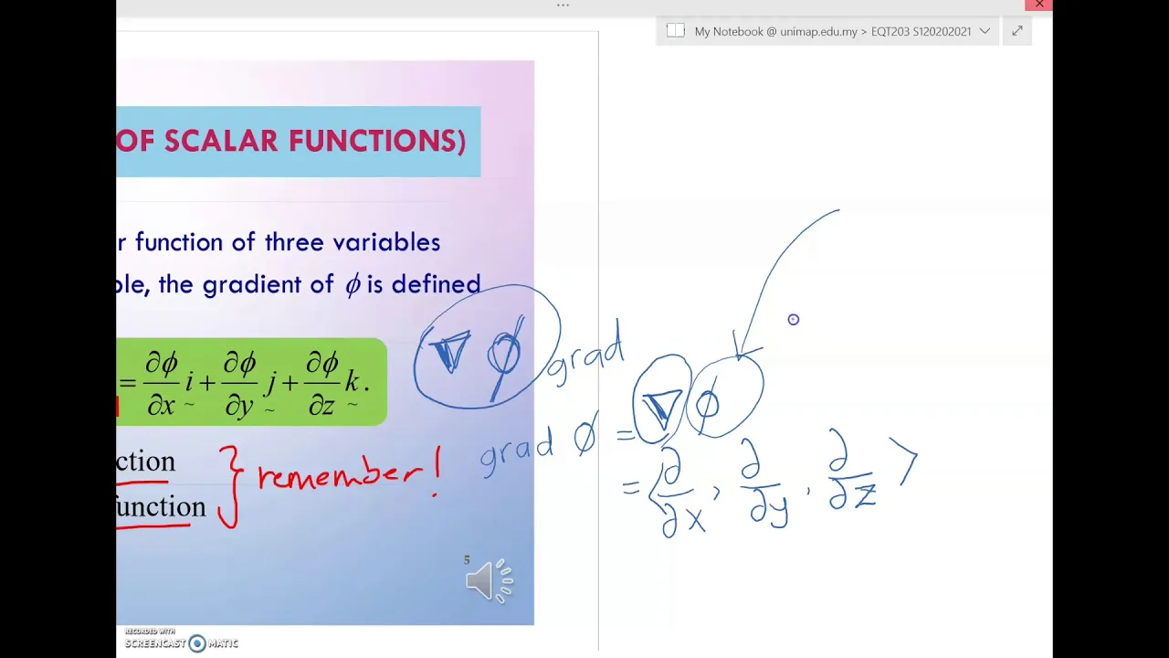
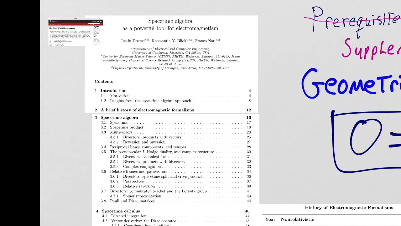
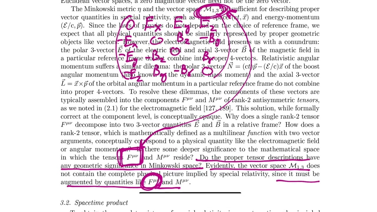
welcome back we are now going to I think today we're going to try to just finish up what we wanted to do we wanted to accomplish a goal in the very beginning of our journey into geometric algebra and SpaceTime algebra our goal was to unify Maxwell's equations meaning I wanted to take let me see if I can find it here I wanted to take the four Vector Maxwell equations that we all learned as undergraduates or in high school these four Vector equations using the classic Gibbs heavyside Vector formulism where the magnetic field is a vector and the electric field is a vector and we just deal with the fact that one of them flips under a change of coordinates one is a pseudo vector and the other is a vector for example polar vector and axial vectors right we deal with all that but we treat everything as vectors and we have four equations describe the electromagnetic field and we compress that into two equations using the formalism of exterior calculus right so now we have DF equals z and the HJ Duel of the exterior derivative of the HJ Duel of the electromagnetic field um form is equal to the current uh one form so this is a let's see this is a two form the hodg Duel of a two form is a two form the exterior derivative of a two form is a three form and the Hodge Duel of a three form is a one form so this is the one form sometimes by the way you'll see it written like this without that uh first Hodge duel and in that case the uh the current is a defined to be a three form I think Wikipedia actually does it that way anyway so we got these four broken down into two which is nice and then there was another section where we had we were also able to break it down into two equations using the the Loren invariant relativistic formulation of of electromagnetism with the electromagnetic magnetic uh tensor and we got it into two expressions and also I think you'll often see this second expression which is kind of complicated by this strange notation of a full fully anti- symmetrized sum but if you take the Dual of F and create G as the Dual of f using using the standard prescription intenser calculus for creating a duel then you end up with a nice simple form so you end up with just this guy and this guy right and remember our goal was to then take these two you know we've got we we found it break broke it down into two mathematical formalisms that have two only two equations for Maxwell's equations we're wondering couldn't we make it one and could we compress these two into a single one and the answer is yes and the answer is geometric algebra and we started our journey in GE geometric algebra with that goal in mind and we studied our geometric algebra but now it's time to just get to this goal the problem is however is there's still quite a bit between us and the goal right the entire this entire section about SpaceTime calculus is actually uh it's it's very rich and I think though that instead of going through it with as much specificity and detailed formalism as we did in the previous sections we're going to kind of cut to the chase a little bit and I will consider doing the heavy formalism stuff in a separate series of lectures just on geometric calculus because it isn't geometric calculus is a fascinating subject in of itself but we can actually get to Maxwell's equations in a vacuum and Maxwell's equations with sources which is our ultimate goal taking all of Maxwell's equations and compressing it into one statement without uh without studying this section on potential representations and without really digging too deeply into SpaceTime calculus as it's presented here and by the way as it's presented here it's it's it's a little too much this paper is a review paper that can't possibly teach SpaceTime calculus in a full and robust way and we would have to leave this paper for a long time and then come back and then this would be super anticlimactic so we're going to try to compress this entire section into this lecture and just cut to the Chase and then come back and address the formalism in another section of lecture so we can think of this as a highle view but we're not going to be trivial about it but we're not going to go into the full depth in detail okay so let's begin I'm going to just Begin by defining the important object this Dell operator in geometric calculus you've seen a Dell operator in regular calculus and when we talk about that Dell operator there's usually an arrow over the top of it and we're going to maintain that convention and you'll see when we introduce that arrow in a moment but for now that for the geometric calculus Dell operator there is no Arrow over it and look at its definition it's very interesting because what we have is we have a unit the four SpaceTime unit vectors right that's what these gamas are this that is the the unit vectors in our SpaceTime algebra and then we have these four partial differential operators each with a subscript and so we're creating an interesting object here it's not a literal member of our geometric algebra C13 it is not a member of that and it's not a member because because these guys here are differential operators they're not real numbers however we are still using these Vector Parts which each of these individually are in fact a member of C13 every one of these uh differential no not differential operators every one of the basis factors are the basis factors of C13 but the differ IAL operators are not uh scalers they're not scalers they're differential operators so we've created an object that has algebraic properties of a one a grade one object right so the algebraic properties of this will mimic a grade one object but it also has this calculus piece that we have to talk about and we treat it very much like a grade one object because look we're going to just use the regular summation convention and we typically will put or I prefer I've seen it done both ways but I prefer to put the vector part in front right normally if we had a literal grade run object we would write you know some component well I guess it would be you know X1 uh uh gamma 0 right plus X2 or or X I'm sorry x0 gamma 0 plus X1 Gamma 1 Etc where the component comes first and the unit Vector comes second that's our typical way of doing things but in this case we don't want anybody to think that you might be applying this operator to this unit Vector because you can't do that that's not how this is going to work and you'll see why in a moment but that confusion is just too much to bear so uh I prefer to put the unit vectors uh in front of the differential operator and now we have this open space where we're waiting to act on something so this differential operator is waiting to act on something and now we need to talk about well what kind of things can possibly go here and what do they mean and it's not an easy question and the paper uh that we're studying really jumps to the hardest possible answer talking about manifolds and and fiber bundles and Clifford bundles and I just don't think we need to go there to get where we want to go which is to unify our Maxs equations so uh we're going to take a simplified approach which the paper actually does ultimately get to anyway and uh just address now our our the new question we have now that we've defined our op our Dell operator is what kind of things does it act on so let's talk about that all right so let's consider a multiv vector which is an element of C13 and remember C13 three is our notation for the entire the entire geometric algebra and the 1 three represents the basis or the uh metric the signature of the metric so our metric has a plus minus minus minus signature is what what that's telling us and so we're considering a multiv vector just in our geometric algebra now the functions that we want to operate on right in other words the functions that we're going to feed in into these differential operators are multiv vector valued functions meaning you put in an input you give it some input X and the output is a multiv vector it's an element of C13 also right so now we've taken our multiv vector and we've kind of turned it into a function and the output is pretty simple to understand right the output is a multiv vector some element of C13 which means it's going to have some scalar part plus some Vector part plus some bi Vector part plus some Tri Vector part which I'll write as the Dual of a scalar part or the Dual of a vector part plus some uh where where W is a vector right plus some pseudoscalar part which we write as beta I where beta is a scalar right so that's a scalar that's a scalar that's a vector that's a vector that's a bi vector and ultimately this is the Dual of a vector so it's a tri vector and this is the Dual of a scaler which is a pseudo scalar so just as a reminder right that's a general multiv vector and this function puts out something like that depending on some input X so now ultimately we're talking about doing things like this gamma mu partial mu M of X right so this partial mu right that's to be understood as partial partial X mu generally where X is some sort of independent variable so clearly this independent variable that if we're to understand this partial derivative the way we normally do this independent variable has to be associated with what is inside of these braces here so what actually is X going to be what are we going to put in to M to get a multiv vector and there's a lot of art to this but we're going to take the simpler approach right there's two approaches one is to Define A Spacetime manifold with coordinates and of course those coordinates would be X mu and every point in the SpaceTime we will erect a separate version of the Clifford algebra and so there'll be a version of the Clifford algebra at every conceivable point in SpaceTime and then we have to do quite a bit of of we we well basically we're creating a fiber bundle of Clifford algebras or of of geometric algebras over A Spacetime manifold and the paper actually talks about this right right I'll show you right here right formly speaking we replicate the SpaceTime algebra at every point in x on a flat manifold so that acts is a tangent algebra with the multiv vector where multiv vectors can be locally defined I'm not going to go through all of that that that is part of um our lecture series on what is a manifold so we're going to not engage with it on that level we're going to engage with it on a slightly simpler level what we're going to do is we're going to say okay our SpaceTime we're going to say our SpaceTime has the spatial parts and the time part right so there's a Time axis this should be four dimensions and everything that sits in SpaceTime can be located with a position vector and that position vector is going to be X mu gamma mu right that is now a position Vector for every point in space time and this position Vector is an element of our geometric algebra so we are giving POS uh physical relevance to certain vectors inside the geometric algebra we are modeling our space time with position vectors and each point will be defined exclusively through these coefficients which would count as the coordinates of the point and this is the unit vectors that establish these axes right the various axes are established by the unit vectors and so the function M that returns a multiv vector is now space time dependent because we are going to write m is a function of these vectors X but the vectors X can be written as X mu gamma mu but mu is this constant object that constructs M itself so it's totally safe to say that m is a function of just the components of the vector that we insert here so we insert a vector but then we sort of rearrange the functions internal guts so that we're really looking at just the components so we've created a way of putting in SpaceTime coordinates inside our function using this notion of a position vector and everything stays inside the geometric algebra that we're dealing with so we don't have to worry too much about this idea of a manifold ultimately we we will get there but not in this lecture so now if I write Dell acting on M I am this is what I mean I mean gamma zero whoops I mean gamma mu partial mu acting on M which is a function of X new gam well let's just say a function of X new right and that equals and that equals uh this uh sum the sum blowing up the sum you we get this expression and it looks like we're doing pretty well here right it looks like we now have an operator operating on a function where the dependent variables match right so I could if I wanted to take this even further I could write D dx0 of M right and Etc I got to be very careful my gamas if I if I draw my gamas too fast they tend to start looking like partials and my if I draw my it's really more of a problem with the partials I'll draw the partials too fast and they'll look like gamas so it's a it's a bit of a mess right but um the point is is that this now starts to look like it's making sense I'm taking the partial derivative of a multiv vector function with respect to a scalar argument that scalar argument is the components of the vector that is driving the position in our SpaceTime so now I have a way of taking derivatives with respect to space time now the problem is is this is still a multiv vector and understanding how to take the derivative of a multiv vector isn't super obvious so let's start with the simplest possible case and uh uh go up from there you know before we get get to that actually let's put a pin in what how these derivatives are actually taken for a moment let's presume that we know how to do that but uh we'll get back to it in a second I want to talk first about some of the algebraic properties of this derivative operator of of the geometric algebra or the geometric derivative we're going to call that the geometric derivative and uh let's begin with the idea of factoring out a gamma 0er we're going to factor out gamma 0er from this expression which won't be hard the first term it'll just pop right out the second term we're going to have to use the fact that gamma 0 gamma 0 equals 1 right so we're going to leave a gamma zero behind when we Factor it out and what is that going to look like well it's going to look like this here's our geometric derivative we take the gamma 0er out on the left side so we leave leave behind a partial zero but here we've added a term gamma gamma 0 gamma zero term and we took the first one out and we brought it out front and we left a gamma zero behind so this expression here what that means as a reminder is gamma 0 Gamma 1 so we write that as gamma 01 and likewise gamma 02 is Left Behind in gamma 03 is left behind but we immediately recognize these guys as as Sigma 1 Sigma 2 and sigma 3 the relative unit vectors so these are actually remember B vectors in the G the SpaceTime algebra but they are relative unit vectors and grade one objects in the three-dimensional algebra now likewise we can do this and that's just a reminder right we're this a lot all this should be total review the tricky part is to understand that these guys just aren't real numbers anymore that's the part we have to get our head around now you can also take the gamma zero out on the right side and you get the same kind of expression except now you end up with the negatives right the negatives of these relative vectors so ultimately you have two forms for this factorization you have the left factorization and you have the right factorization and the right factorization we introduce this negative sign to correct for these uh superscripts to flip the superscripts you have to introduce negative signs everywhere so that's what we have we have these two terms but what we're going to do is I'm going to take this guy and I'm going to say you know what that's a three-dimensional unit vector and a regular partial derivative we're just going to call that the gradient operator the three gradient that's what that is that's the three gradient so this now becomes these two expressions right becomes the time partial derivative and the three gradient and the time partial derivative minus the three gradient depending on whether you factored out to the left or the right which reveals the algebraic structure of our geometric derivative expression you're starting to see we're treating it just like a member of the algebra and what the paper likes to point out that is I'm not quite sure how profound it is but the paper says well you know we've got the gradient operator which treating it like a one object so we should be able to take the geometric product of that thing with itself which we can write as um geometric derivative squared which is going to be just this guy multiplied by that guy right and there that is written out and of course this immediately goes away because gamma 0^ SAR is+ one in our convention so now you have this look what you're left behind you're left behind the uh the same two objects summed one is summed and one is is subtracted one is added and one is subtracted which of course is the way you factor something that is square you you it's the it's the uh factorization of x^2 minus y^2 right you know it's the X + Y and the xus Y right so what's interesting is but here we have the Ware of something which mimics this structure when once you get rid of this and what is that ultimately leave us with and It ultimately leaves us with what we know to be the D ersion of regular of our regular Vector approach but now the Dal ersion factors into a single perfect square which is evidently I mean that's what Direct kind of wanted to do when he created his formalism he had to go through some tricky mathematics to find a way to get something that was the looked like the square root of the dersin so he could create uh a a a structure for the electron based on this this notion very important idea I think but uh it is sort of beautiful to see that this very Elementary algebraic steps get you something that looks like the square root of the dalish uh but regardless even if that escapes you or doesn't seem that profound to you this algebraic step is still relatively important it connects our geometric algebra notion in the SpaceTime algebra with our physics Notions and our relative algebra that we've been working with okay so I think that covers most of the important algebraic steps oh there is one other you want to say okay well we can also if we're treating this thing seriously like a member of the geometric Algebra I can ask well what's the wedge product of it with say gamma 0er and that wedge product is going to be pretty obvious right right we'll just take this wedge straight up and we end up with gamma 0o wedge gamma 0er so we know that that is going to immediately go to zero remember we're treating this like a scalar oh that should be a zero we're treating this like it's a scalar object so um it's doesn't participate in this wedging and then we end up with these gamma Zer gamma I which is just Sigma I and uh ultimately this just equals our three gradient right and likewise uh gamma 0 dot Dell or dot our geometric derivative is just going to be the partial with respect to zero so there's more out so those and there's probably more algebraic relationships that are important here but we're just trying to get used to the idea of treating our geometric uh our geometric derivative right which is you know this guy right here as an algebraic object setting aside the fact that we have derivatives for their components okay so what next okay so now let's take the consider the derivative of a scalar function so the input is still going to be a position vector or a vector as we understand a a four-dimensional vector in our geometric algebra but the output is just a scalar so this still counts as a multiv vector function because remember a multiv vector function has a scalar Vector bi Vector Tri vector and pseudoscalar part at least in the space-time algebra but um yeah just consider one that only has the scalar part that still counts as a multiv vector just as a reminder so there's our multiv VOR and now we just create this object so I'm going to make my substitution for Delta now the substitution I like to make for the purposes of our SpaceTime algebra is this substitution here when we study the general geometric algebra which is I think what I'll eventually do in a separate series of lectures we're not going to have this we're not going to immediately drop into this sort of convenient notation it this really only works for the SpaceTime algebra uh or is only used in the SpaceTime algebra and a lot of it is used just to give us the comfort of seeing things we recognize from our regular work which is one of my criticisms of this is we're actually leaning on our old stuff a lot here but I I feel like it is the way to go um so I'm going to make the substitution for the geometric derivative with this factored form and then that will give us this form when we move Alpha which is a function of X I'm suppressing the X here into the operator so this be this is the gradient the three gradient operator and this is just the time partial time derivative so this is easy to understand because this is a scalar function of X and and x0 is a regular real number so we we know exactly how this derivative is regular calculus right here and this is also regular multivariable calculus but if we look at it in terms of the geometric algebra we have this becomes Sigma 1 partial 1 Sigma 2 partial 2 Sigma 3 partial 3 and Alpha and we know each of these is just a function of a real variable and it's the partial derivative of a function of a real variable so each of these are real numbers these are B vectors however we treat them as uh just regular vectors in the three-dimensional algebra and But ultimately this ends up being a b Vector well does that make sense that this would this part would be a bi Vector well sure because we're now going to take this B Vector is geometric product with gamma zero but each of these terms has a gamma zero leading in the B Vector right so we have we have gamma 0er geometric product with something that looks like gamma 0er wedge gamma I right so this wedge this geometric product is going to ultimately just kill the gamma zero and you're going to be left with a gamma I so what we have is an object that has the algebraic properties of a vector which is our geometric derivative multiplied by a scalar which should be a vector and that's exactly what we get this guy times this gamma 0 is a vector this part is purely scalar so times a vector is also a vector so we end up with a uh a vector exactly as we would expect just by looking at this uh at this basically a geometric product of a vector with a scalar so that one's pretty easy to understand all right now let's consider a vector function where the input is a vector and the output is also a vector now remember the input we're considering a position Vector in our SpaceTime model but this output could be any other Vector so we're looking for the geometric gradient or the geometric derivative of this Vector function where now I've suppressed the variable X right here and let just first before we really dig in let's well we I guess we are digging in but let's just blow this thing up and see if we can get any more insight regarding how our geometric derivative actually acts like a one grade object so I'm going to make the direct substitution right so this part here is directly the definition of that of the geometric derivative and the vector we're just going to blow up into its components right here right so we those the two pieces of of our geometric derivative of this Vector function then uh we are going to commute the things that look and behave like scalars in this case this is a scalar this V is a scalar and this is a derivative operator and this is a function right these are remember this this guy V of X is a function but it does return a vector and that Vector is ultimately V mu gamma mu right so these guys here are also functions of the coordinates so this is a partial derivative of a function so we can actually take that partial derivative in principle given mu and new we could take that derivative um the uh because this guy here is a scalar right it's a component of a vector so it's a scalar so all of the algebraic properties reside in this expression this geometric property of these basis vectors and their dual so if we blow that up we know the geometric product of these two things is going to be this this uh inner product plus this outer product right that's a fundamental thing of two two uh vectors in the geometric algebra multiplied together it can be broken up into this symmetric part and this anti-symmetric part which we defined as the inner product and the outer product and then our partial derivative lives outside the brackets but this because we're dealing with the vector and its dual here we'll get this Delta function mu new and then I'll bring I'll bring this piece back in over here so we have this Delta function and we have this derivative and then here uh I left this part alone uh I guess I guess what I needed to do was get rid of these brackets here right so now it looks like uh we have this outer product multipli by what is a scalar process right this is going to be the partial derivative of a scalar function so that's scalar so this is a bi Vector piece and this is a vector piece then I execute this Delta function and we're left with uh the partial Mew and the sub superscript here is Mu so that is just a uh uh that is just a a Divergence really but it's going to ultimately be this expression this Dell Dov right this dell. V if you execute the algebra of Dell Dov you get this expression and here if I now move this guy to become the coefficient I move our scalar piece to become the coefficient of this part I end up with the definition of the derivative and I I leave the vector part behind and this reconstructs the full vector v and this reconstructs Dell so I get uh uh this reconstructs um the geometric derivative so I get this piece I get the anti-symmetric part and that is exactly how you would expect an object a grade one object acting on a vector to behave if that's a grade one object and that's a vector the geometric product has the same form we've always used to expect so that's totally cool so that's just I'm just sort of breaking down the more of the algebraic nature of this Dell operator but let's take a closer look on how this product would actually manifest itself so to demonstrate this we're just going to make direct substitutions for what we know to be the algebraic structure of the gradient oper of the geometric der ative and a vector so the geometric derivative we're just going to immediately substitute this known form right here and you might say well wait a minute in the known form we did the zero was up there but remember in our convention gamma 0 uh gamma 0 gamma 0er that equals one by definition actually and uh between that and this fact that gamma 0 geometric product gamma 0 equals 1 we know that gamma 0 equals gamma subscript 0 equals gamma superscript 0 so we can make that arbitrary change on the other side we have uh V equals uh uh V uh we we'll we'll we'll write V in the um uh yeah I guess we'll write it in the normal form V 0 V V v0 gamma 0 plus VI gamma I and then we factor out a gamma Zero from this so once once we have this we can factor out a gamma Zer so we'll get gamma Subzero V superscript zero and we have to we since we're we have gamma 0 gamma 0 equals one so we have to leave a gamma zero behind so we'll end up with gamma 0 gamma i v i like that but this is minus Sigma I so we end up with gamma 0 v0 minus the vector the relative vector v right so that's exactly what we want right here and uh oh it's not exactly because here we have a subscript zero and here we have a superscript zero but again in our convention with our metric this the zero component can be exchanged uh arbitrarily with subscript and superscript so we just dro the superscript and this matches what is done in our paper okay so now we're going to blow this up and we're going to get a very simple expansion now the we have to remember a couple things this is we've done this before when we first studied relative vectors right relative vectors live and operate in a threedimensional geometric algebra and this guy over here is clearly in our SpaceTime algebra sta is a typical abbreviation for SpaceTime algebra so we want to take advantage of the fact that we have this three-dimensional SpaceTime algebra to work work with so typically just as a reminder when we think of the basis vectors gamma mu for the SpaceTime algebra with a metric with a signature with a metric signature one minus one minus one minus one right right that's our sort of metric signature and we think of the three-dimensional uh algebra as just Sigma I with a complete one one metric right and these guys are regular vectors they're grade one objects they're one grade objects in the 3D algebra but they're by vectors in the SpaceTime Algebra I know we've gone through this a lot but it always confuses me so I assume it confuses everybody that's probably a bad assumption but so we're going to treat this process up here as much as we can inside this threedimensional geometric algebra so when I see an object like this this gradient object this uh three gradient well that's Sigma I partial I that is a vector in the three-dimensional algebra it's a bi Vector in the SpaceTime algebra but it's a vector in the three-dimensional algebra this V with a bar over it well that we constructed to be a vector in the three-dimensional algebra so this concept this thing this thing is now um Sigma J V with a little J there this object here is the product of a vector times a vector in the three-dimensional algebra it's also a bi Vector product in the SpaceTime algebra fair enough but we're going to work as much as we can in the threedimensional algebra because it's a lot it's actually a bit easier but also we're headed that way we're trying to up with Maxwell's equation so we want everything to look like threedimensional vectors as much as we can and we're making some progress okay so with that aside let's move on and we're going to immediately take advantage of this what I just said by treating this as a geometric product of two vectors so this is going to immediately blow up into this inner product plus this wedge product right because it's two vectors right so that's what that's the definition of the geometric product of two vectors it's got a grade lowering piece or a symmetric part A symmetric grade lower and a symmet anti- symmetric grade higher piece and that's exactly what we're going to do and now I'm going to take all of this stuff and we're going to mix it by U by by quality by type for example that is the partial derivative of the component of a vector so this thing is a scalar it's a scalar function you got to remember now V is a function of this Vector this you know this inserted Vector mu so V is a function of SpaceTime in the sense that we've defined space time to be a position Vector as the argument of our function so i' I've in other words I've suppressed X this should read Delta VX 0 X1 X2 X3 like that so this partial derivative is the partial derivative of a scalar um or is the partial derivative of a scaler because we're now looking at the v0 component of this object right so this is a scalar that's my my point there so I will Circle that in red because it's a scalar now this next next object is the partial derivative of a vector so if you just blew that up You' have the partial derivative of an object that looks like um v0 gamma 0 plus V1 Gamma 1 Etc right so you end up taking partial derivatives of the components but you're not taking partial derivatives of these unit vectors so you're leaving the unit vectors behind so this object here is a vector object it's a vector object remember all in the 3D right we're thinking in the 3D now it seems weird we're thinking in the 3D in terms of the algebraic property but notice this subscript is still the time subscript of the SpaceTime algebra right so it's a it's a little bit delicate there um but uh not so bad I can track all that so let's keep going and now we're going to study this part well this is a a vector multiplied by an object that's a scalar so this is obviously a vector right this is obviously a vector this has the AL the the U this three gradient has the algebraic properties of a vector in the three-dimensional algebra so that is a vector and that leads us with well these two parts this is a vector dotted with another Vector clearly that's a scalar and this is a vector dotted with a uh Vector so this is a bi Vector so I'm going to circle this part here in red because it's a scalar and then this bi Vector part I'll Circle in blue okay so now we've kind of chunked up now I'm going to reorganize it so it's organized by grade so here's the grade organization this is the scalar part this is the vector part this is the bi Vector part now let's consider I I really I hate to do this because I know I'm going to screw it up but remember our original piece here is the gradient is is the uh geometric derivative of a vector and we've decided already that this acts like this guy here already acts G algebraically like a vector so this thing really needs to be in the SpaceTime algebra Dell Dov plus d wedge V right and this part is scalar and this part is by Vector in the SpaceTime algebra and that's not an ju and just to be clear that's not too demanding in the sense that well that's scaler for sure and these two are not scalers for sure so this part is definitely linked to that part but let's make sure that the rest of this stuff is A Spacetime B Vector so we can link it to this piece now the this first part here the part in green well these are 3D vectors but we know 3D vectors are composed of objects that look like Sigma I or Sigma lowercase i which would be gamma 0 I or gamma i0 right so these guys are in fact SpaceTime by vectors no problem so the green definitely um belongs in this grouping the space-time B vectors now this part it it doesn't take too much thought it would look like you're dealing with a you're dealing with a B Vector right times uh wedged with a bi Vector so you think that this might be a pseudoscalar and and I even made this mistake myself a couple times but it turns out that you're it's it's always going to be a bi Vector of the form Sigma uh Sigma I Sigma J something like this right which is always going to be uh gamma z i gamma j0 and by the time time you work through all of this the you these are geometric products so this is going to be gamma 0 gamma I gamma I gamma 0er right and then we know that the gamma zero we could just lift and the gamma I we can lift if we add a negative sign and then we commute this zero through twice get rid of it and we have oh this should be a j I think a j yes sorry this should be a j and um the point being is that we're always left with a gamma i j we're always left with a bi Vector so it as a matter of of practicality for this calculation this piece that looked like it might have pseudoscalar potential isn't it's always a bi Vector so it always belongs in there and so what we're seeing now is that we've got this is a total Divergence in the SpaceTime algebra and this part represents some kind of generalization of the curl uh in the SpaceTime algebra using the geometric algebra um that's a little less obvious until you substitute this away and we're looking now remember we want to lean on our 3D geometric algebra so we want this to look like a cross product so let's see if we can get this to look like the cross product which is not very hard we the first thing is we remember the definition that in the 3D geometric algebra if I have two vectors A and B the cross product that we're so familiar with is the wedge product multiplied by the inverse of the pseudoscalar so it's a it's a dual of the wedge product so the wedge product is a b Vector it's dual that means the part of it that doesn't have this minus one on it that would be the Duel of it but you uh we we Define it with the uh the inverse there so and usually in in in the space in the algebras we deal with i^ s equals -1 so I inverse equals minus I so sometimes you will see this written this way if they're talking about a particular SpaceTime algebra for example but the point is is that the wedge product is this cross product which remember the cross product in uh regular gibsi and stuff is a vector so the Dual of a vector is a bi Vector so that's what we have we have a b Vector on the right and the Dual of a vector on the left makes perfect sense so this guy here can now be substituted away like this we at we now have this term Dell cross V now that cross needs to be a unambiguously a cross it kind of looks like a a variable X so I want the cross product right now I could put parentheses here but the standard rule is geometric products are always done last so this cross product would be done first and so this the order of operations makes this notation uh this notation right here just fine so now I have AC I've actually introduced a cross product oops I guess one part thing I'm missing is a little Vector over the V to make sure you know it's a relative vector those arrows are actually really important now so this expression uh our final version of this expression looks like this right here okay so that is how we take the geometric derivative of a vector in the SpaceTime algebra okay so that's where the fun began but now this is where the fun really takes off because because we are now interested in the geometric derivative of B Vector fields and the reason this is now important is we have to remember our electromagnetic field we want to model as a bi Vector field so the electromagnetic field by Vector is going to we're going to write everything down very suggestive notation now so e is uh is going to be a relative vector is given by EI Sigma I so this is a b Vector in the SpaceTime algebra but we're writing it down as a relative vector and b is another relative Vector but the f is going to be the sum of the of the two but B it's going to be the Dual of B and what that just as a reminder how that works is all of the sigma I are defined as gamma zer gamma I but what we are looking for for um the magnetic field is always the Duel of this in other words we always need uh the magnetic fields always have to be uh something like Sigma uh J gamma J gamma K gamma J gamma K both spatial right there's no gamma zeros in the uh in in the magnetic portion of the magnetic field tensor so we're going to model ultimately the magnetic field as a vector in the three-dimensional geometric algebra but when we start working with it we're taking its dual and we're adding it to the electric field which is a relative vector and we end up with our model for the electromagnetic field tensor this is a bi Vector right it's always going to be a bi Vector because the Dual of a b Vector is a b Vector this is a bi vector by definition e is a b vector by definition so now we're looking for the derivative of f so let's play around with that well here we go we are taking the geometric derivative of a b Vector F let's just treat everything algebraically and see how far we can get we're going to substitute this expression right here on the left hand side for the geometric derivative so we have this scalar operator and this relative Vector operator and on the right hand side well that's what f is f is this by Vector when I and you know we're I know we're going to run into this problem over and over again it's a bi Vector in the space-time algebra it is a um but what it's what it is in the uh 3D algebra this is a vector in the 3D algebra and this is a b Vector in the 3D algebra because it's the Dual of a VOR Vector in the 3D algebra but in the uh SpaceTime algebra this whole thing is all one big by Vector okay so with that in mind now we just multiply this thing out and we do the obvious thing we get this partial derivative this first term then we have these two cross terms and then we have the final term and notice that uh this pseudo scaler just follows everything like it's a constant everything it just follows through this problem like a constant and the next step is to treat it like a constant now I'm going to pull out the pseudoscalar where I find them so the pseudoscalar exists here and the pseudoscalar exists here but anyway the first term doesn't change the second term I just sort of pull out the pseudoscalar because it's not subject to the derivative and in these two cases we have these derivatives of vectors but we know how to do that right because the vector e is is just going to be e0 Sigma well not e0 right because this is a this is in the 3D algebra E1 Sigma 1 plus E2 uh Sigma 2 plus E3 Sigma 3 and E1 is a function of X and that's a derivative of that argument so we're going to be taking the derivatives of these component terms and what's going to be left behind is a vector so inside inside these braces I guess there's another bracket over here I forgotten because this whole thing is multiplied by gamma zero right so inside these brackets this is a vector it's a vector but the derivatives that we're taking are always derivatives of scalar functions likewise this is a vector uh the the derivative of B is a vector but it's going to be the Dual of that ultimately right so the that will ultimately look like a tri Vector in the SpaceTime algebra and a b Vector in the uh 3D algebra this should uh ultimately be in the 3D algebra a scalar term right this has got to be a scalar this is going to be a uh a b Vector in the 3D algebra this is going to be a scalar in the 3D algebra and this is going to be a bi Vector in the 3D algebra and now we can start seeing Maxwell's equations in here right if we treat our electric field and magnetic field literally with E and B well we have a Time derivative of the electric field we have a Time derivative of the magnetic field we have a to a Divergence of the electric field and a Divergence of the magnetic field and we have a wedge product here and here but we just saw how to convert wedge products to cross products so we have a curl of the electric field and a curl of the magnetic field so we can clearly see that the derivative of f when it's decomposed has all the pieces of Maxwell's equations inside it and that is very exciting because clearly that is how we're going to get to our final goal which we're zeroing in on uh very closely okay so uh what next okay so the next step is going to be to uh rearrange this so we isolate all the terms that are duels meaning we keep all the we take all the factors with the pseudo scaler to the right and we replace all of the wedge products with cross products and that's not so hard I just did it right here this term has uh no no duality no pseudo scalar uh this term has no pseudoscalar this term when I convert it to a cross product will have a pseudo scalar but this term when I convert it to a cross product will introduce a suar scalar which will multiply by the one that's already there giving me a minus one so that accounts for that minus sign so this minus sign here comes from replacing that with uh D cross B I right so you get Del cross b i i and those two I give you a minus one and um then uh obviously this term has a pseudo scaler and that comes right to here right so this term ends up there and this term gets it PT scalar so it comes there and then the Del do B oh wait a minute wait a minute wait a minute that's I've got that backwards right it's this term goes here this term goes there and then this guy obviously has a pseudoscalar goes there and this that's where the pseudoscalar lives so we are all good with those splits and now um so uh what have we got well this is a 3D geometric algebra Vector this is a 3D geometric algebra scalar and this is a 3D geometric algebra bi Vector likewise 3D geometric algebra Vector 3D geometric algebra scalar and 3D geometric algebra b Vector so both of these pieces the piece that's well then then each of these of course is given a 3D Duality transformation so this this um scaler becomes a pseudoscalar this B Vector becomes a Vector right and this Vector becomes a bi Vector so yeah and that's the way we expect we expect magnetic fields to always be bi vectory we expect electric Fields always to be vectory right so um and you can see right in here these are all the parts of Naturals equations these are time derivatives remember gamma zero or partial zero is a is with respect to time time is the zeroth component so here's our our Divergence of a magnetic field of the magnetic field the magnetic Vector field in the 3D algebra there's the Divergence of it there's the curl of the electric field the curl of the magnetic field all of those things show up in maxel equations so now the question is is how do we tease them out to actually look like Maxwell's equations and let's just do it and call it a day so step one we want to reorganize this so that we have the scal parts and the vector parts and the bi Vector Parts in sequence so we can kind of sort them in our head let's do that first okay so that was pretty easy right all we have to do is swap things around I did a little color coding scalar parts are in red Vector parts are in green and when I say Vector I'm talking about the 3D algebra right the 3D algebra so uh now we have uh this is the geometric derivative of our electromagnetic field is written like this so now what do we do next to sort of pull out maxel equations well if we we're looking for a formula right so we're look this is just a definition really all we've done is Define things and move things around we haven't interjected any physical principles in here we're saying our field is modeled by these things and we're calling F the electromagnetic field um uh uh uh bi Vector but we haven't said anything about it we've just this this is the this is true by definition right so if I was going to assert some Physics I might be inclined to do this I might be inclined to say equals zero right so to make it a little bit tighter I might be able to Incline to write the geometric derivative of f equals zero and what will that get me well the first thing it would get me is this side this left hand side is all kinds of different objects right when I say this is a scaler when I say D.B is a scalar I'm actually forgetting about the I it's really a pseudo scaler right it's a pseudo scaler and the only true scaler here is d. e right when I say this is a when I say the time derivative of B plus the curl of e is a vector again I'm forgetting about this I out here it's not a vector it's actually a 3D B Vector right so this part here I'm now going to circle in blue right I'm going to circle this in blue that is a b Vector this pseudo scaler I'm going to circle in uh let's say squiggly blue maybe how about that I'll I'll squiggle it around so that's a pseudo scaler right then this red piece here this really is a scaler and this part here in green really is a vector so I have a bi Vector piece a pseudoscalar piece a vector piece and a [Music] um uh and a a scalar piece now you say oh wait a minute you forgot about this this turns everything upside down this turns your scalers this this gamma zero turns your scalars into vectors your vectors into bi vectors and things like that but remember I'm setting it equal to zero right so I'm going to multiply both sides by gamma zero and I'm going to get rid of this gamma zero right because remember the gamma Zer is actually multiplied by everything you see a factor of gamma 0 here and you see a factor of gamma zero there so that gamma Zer will go away and I'll be left with everything exactly as I described so let's write that out and so once I've done that I end up with the scalar part in red the vector part in green the bi Vector part in blue and the pseudoscalar part in black and each all equals zero and of course the next step is should be somewhat obvious is that in order for this to ever be true each one of these parts has to equal zero by itself by itself so I immediately recreate Maxwell's equations in a vacuum I get D do E equals z i get the time derivative of the electric field minus the cural of the magnetic field equals zero I get the time derivative of the magnetic field plus the curl of the electric field equals zero and since and remember since this term has to equal zero that I just goes away right I end up pulling it you know multiplying both sides by I and dividing through by a negative sign so I get that equaling zero and then I get finally um the legendary and famous dell. b equals Zer and of course in a in a vacuum this is Max's equations in a vacuum and the paper actually cites that right so this is from the paper that we're reading right Max's equations in a vacuum dell. f equals z f is our model for the magnet electromagnetic fields and it's modeled exactly the way I described and they break it down into two parts right you have d f equals z and d curl f equals z um and of course you can this is true because we're dealing with the 3D you know the relative algebra right and But ultimately uh it breaks down exactly the way we broke it down the divergences are both zero and these curls um are completely symmetric but that minus sign is just perfectly there it's it's there and it belongs there so that looks really great so we're almost finished because now we need Maxwell's equations that are not in a vacuum right Maxwell's the the general macel equations that has charge density and current density in it so that that's not a very big step away right all we need is something on the right hand side to model charge and current density and so now we're going to look for a model for charge density and current density and put it on the right hand side and of course that's just going to be yet another uh yet another um piece of the geometric algebra so let's take care of that so the next thing we would think of is okay well if that's Max's equations in a vacuum what if I say it's not in a vacuum and I say there's some current out there and I now model the current density with j a vector J let's go with a vector so J is going to be J mu gamma mu and then we do the usual process J mu gamma mu ultim that's going to be gamma 0 we factor that out and we have uh j0 plus j i Sigma I right so I do the SpaceTime split that we always do and that now becomes my J mu gamma mu well you may remember uh that zero term before that there is a gamma Zer floating around over here so if I put the J over here I have to sort of return that gamma zero over on on the the far left so if I now replace this with its space time split I have a factored gamma zero on both sides and it all goes away so what is that ultimately going to look like and with this all we do is the same thing we did before I guess this is a scalar part and this is a vector part so the only thing that changes now is I have Delta E equals what we're going to call the j0 piece and that's the scalar part and then the vector part partial z e minus the curl of b equals J I right that'll be the vector part well I guess I should write that a little more this wouldn't be ji it would just be J the3 Vector right because this is now this is actually equal to uh the red part being the scalar j0 and then the green part plus J the vector piece right and then these two actually remain the same right you still get you still get the curl of b equals zero because there's no pseudoscalar part over here and there's also no B Vector part so you still have uh you still have the time derivative of the electric field Vector um plus the curl of the electric field equals zero and so now it's just a matter of connecting J to the units that you're choosing right so for example I will go to the the paper that we're actually reading they do that um they do it they they the paper where really takes a few extra steps to get to where we want to be they include magnetic current and a few other things so how how would that translate let's take a quick look right so a you in in their formula in the formulation in the paper they include magnetic charges right so I'm not going to worry about that so let's get rid of some of that stuff and they also use a part of a potential formulation in their explanation which we didn't need because we're just demonstrating this so with no magnetic charges right this of course goes to zero with no magnetic charges there can be no magnetic current and so that goes to zero and then you're just left with the units that you choose right and they're choosing the units um you know they they have a factor of C Works in there remember our derivatives our our Subzero derivative uh is all is the same units as space I I wouldn't worry too much about the units they they do do a very nice job of helping with the units in the paper if you really really care about it but just understand we don't we did when our analysis we didn't go through this potential formulation that they did which is pretty interesting but um uh it's not super relevant oh I do notice a mistake we made right see the minus J there the minus J that's important right what did I do hold on a second yeah see remember when we when we take out this gamma zero that should be a minus sign right so that should be a minus sign let me erase that change it to a minus sign which means this here is a minus sign and ultimately the minus sign Finds Its way right down into the equation itself so that should be a minus sign and I think that will agree with what they wrote here uh time derivative of the electric field minus the curl of the magnetic field is the opposite of the current the electric current and is that what we have uh we have we have the yes that's exactly what we have so there you have it so ultimately now we can write D or the geometric derivative of f equals J and with that we can go back to our first page and this was over an hour ago but you remember this right here's our here's our maxel equations in fullblown form here's our uh here's our uh exterior calculus form here is our Loren's inv variant relativistic form and this is the missing magic thing that we finally after all this time are able to write d f equals J right and this is a four vector and this is the electromagnetic field by Vector right and this is the geometric derivative and there you have it we've got it down to one little formula so that was a long journey and I am going to call this mission complete meaning I probably will not be returning to the rest of the juicy stuff in this paper uh it was delightful I do plan to study this in a separate class I think I'm going to redo all of geometric algebra in a new context maybe using some new software that I've got and I've learned how to use but look at how much more material is in here I mean this is a 100 page paper and we really left out some juicy stuff but to get to where we wanted to go the hard part was just learning about SpaceTime algebra and we did a very thorough job so thank you for sticking with this lecture series and I hope to see you in the next one
Up Next
23:39
Vector Derivative in Geometric Calculus: Gradient and Maxwell's Equations
@AlanMacdonald1
12.8K views•2016-03-19
9:28
Maxwell's Equations in Geometric Algebra | Multivector Form
@PeeterJoot
13.5K views•2023-10-30

32:32
NMR Spin Physics I: Zeeman Effect, Resonance Condition & Larmor Frequency
@nptel-indianinstituteofsci8064
2.3K views•2024-01-17

33:44
The Blue LED: A Decade-Long Scientific Challenge Explained
@veritasium
46.5M views•2024-02-08
Related Study Plans & Knowledge Roadmaps
Structured learning paths in Physics
physics
Medical Physics: Imaging, MRI & Radiotherapy
01Foundations of Radiation and Matter Interaction
02X-Ray Imaging and Computed Tomography (CT)
03Magnetic Resonance Imaging (MRI) Physics
+ 3 more learning modules
15h6 modules
Explore Roadmap
physics
Nuclear Physics (Decay, Fission & Reactors)
01Atomic Structure and the Binding Force
02Radioactive Decay and Half-Life
03Nuclear Fission Mechanics and Chain Reactions
+ 2 more learning modules
12h5 modules
Explore Roadmap
physics
Soft Matter (Polymers, Colloids & Rheology)
01Foundations of Soft Matter & Thermal Forces
02Polymer Physics and Macromolecules
03Colloids, Surfactants, and Self-Assembly
+ 2 more learning modules
38h5 modules
Explore Roadmap
physics
Analytical Mechanics: Lagrangian & Hamiltonian
01Mathematical Foundations: Calculus of Variations
02From Newtonian Mechanics to Constraint Dynamics
03The Principle of Least Action & Lagrangian Mechanics
+ 3 more learning modules
28h6 modules
Explore Roadmap