




![Div, Grad, and Curl: Vector Calculus Building Blocks for PDEs [Divergence, Gradient, and Curl]](https://i.ytimg.com/vi/lKXW7DRyyro/maxresdefault.jpg)




![[전기기초 3편] 전기가 처음이라면 꼭 봐주세요! - 전기기능사, 전기산업기사, 전기기사](https://i.ytimg.com/vi_webp/fZ5-GOOnJzM/maxresdefault.webp)
![[전기기술사][전자기학 1강] 전기력, 전위, 전위차에 대하여](https://i.ytimg.com/vi_webp/y_KXoftZRQQ/maxresdefault.webp)


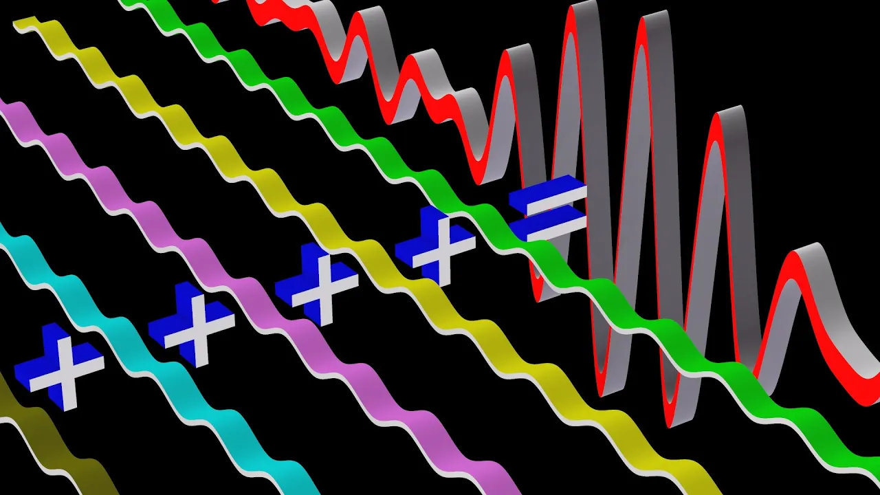


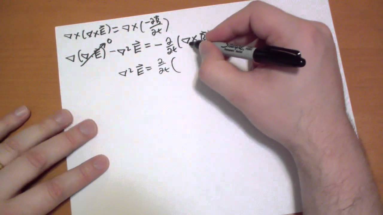





The wave equation for electromagnetic waves is derived by combining Maxwell's curl equations (∇×E = -∂B/∂t and ∇×H = ∂D/∂t + J) and applying vector calculus identities, resulting in ∇²E = μ₀ε₀∂²E/∂t² for free space, where the wave velocity is v = 1/√(μ₀ε₀) = c (speed of light). In dielectric media, the equation becomes ∇²E = μ₀ε₀(1 + χ)∂²E/∂t², where the refractive index n = √(1 + χ) determines the wave velocity as v = c/n. This demonstrates how electromagnetic waves propagate at different speeds depending on the material's permittivity, with plane wave solutions showing electric and magnetic fields perpendicular to each other and to the propagation direction.
Deriving the Wave Equation: Plane Waves & Refractive Index in Optics
Added:Maxwell's Equations in differential form, which serve as the foundation for deriving the electromagnetic wave equations.
Vector calculus operations, specifically curl, divergence, and the vector identity for the curl of a curl.
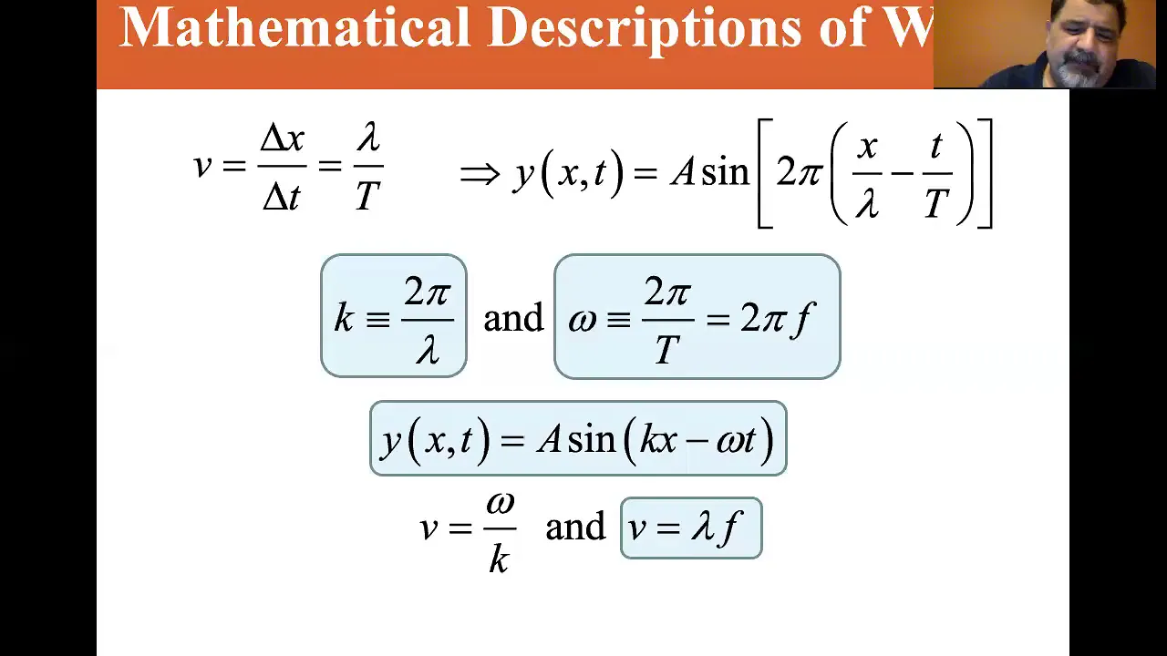
Basic wave mechanics, including concepts of frequency, wavelength, phase velocity, and the general mathematical representation of a traveling wave.
Constitutive relations in electromagnetism, defining how fields interact with dielectric media via permittivity and permeability.
Boundary conditions and the derivation of Fresnel Equations to describe reflection and refraction of plane waves at interfaces.
The physical distinction between phase velocity and group velocity, particularly how dispersion affects wave packets.
Wave propagation in conductive, lossy, or anisotropic media, introducing concepts like skin depth and birefringence.
Applied optical technologies such as waveguide design and fiber optics, which rely on wave confinement and dispersion management.
6.8K views50likes22:35Original Release: 2022-09-26
[Music] hello everyone welcome back uh in the last lecture we were talking about the the scientific problem in nanophotonics so when we have a distribution of uh permittivities in certain region of space how do we solve for the electromagnetic response and mentioned that uh this essentially inv essentially involves solving Maxell equations but how do we solve that so uh to do that we have to essentially solve the wave equation so if you look at the Maxwell's equation the curly equations here you have two of these curl equations curl of H and Cur of e and when you combine these two you get what is known as a wave equation this is a wave equation for uh free space okay so how do we get this equation so since this is a central uh part of nanophotonics I would like to take a little bit of time try to derive this so you might have already done this but I just want to go over this one more time so that uh you familiar with the assumptions that we are making and what is the role of each uh term okay so uh all of you definitely are familiar with wave equation which is of this form this is essentially a second order partial differential equation so you have the second derivative in time this is second derivative in time and sorry uh I have my students here so they're asking me question so let me yeah what is this well why why should it be H it can be electric field as well you can have the electric okay so yeah the wave equation has two forms one is the wave equation in terms of electric field and the other one is the wave equation for the magnetic field so you can have either of these two things we can derive them so it depends yeah so what I'll do today is I'll derive the wave equation for the electric field and I'll leave it as an exercise for you to derive the wave equation of the magnetic field you can do that okay and it'll be similar in form so that's a nice exercise yeah thank you so much Sahan yeah so uh yeah we have the second derivative in time on the right and we have the second derivative in the space so this is a lapian Operator lapian Operator which is essentially do Square by dox S + do Square by do y square + do Square by do Z sare this is a lapli uh operator in the cartisian coordinates so the wave equation essentially relates the second order second derivative in space and in time so through the velocity term so I mean I leave it as a small exercise for you to check that the dimensions match out so the coefficient of here is going to be the velocity term okay this is a wave equation so how do we get this wave equation so we will start with the curl equations given by Maxwell and we'll also make an assumption that the magnetization is essentially zero so we'll only take uh B is going to be mu H mu H okay this is the Assumption we're making so with that I have curl of e which is given by second the partial derivative of B with respect to time and that will be minus uh uh the the partial derivative of the magnetic field with respect to time the second derivation is second equation is simple enough so what we'll do now is we'll take the curl of the first equation so let me take curl of a so what I want to do is take curl so I assume that you have gone through a course on Vector calculus and you know what curl Divergence and all mean if not I would encourage you to take it because these equations this uh Vector calculus is very fundamental to a lot of areas of engineering so you should take I many it will be just a you know monthlong course on Vector calculus you should take it there'll be a lot of resources that are available in that context so let's consider curl of the first equation so I have curl of e so I'll take a curl of that and that on the left hand side so that will give you on the right hand side minus mu I'll take the derivative out and I'll say curl of H right so I know what is Cur of H from the second equation the B here so that will be equal to mu not uh since the this is okay let's take the second derivative so so mu not second derivative of D with respect to time plus the minus mu yeah the first derivative of uh J with respect to time so this is a okay this should be instead of a plus it should be a minus here as well so this is what you get right and you also know that from the constitutive relations we know that D is equal to Epsilon e+ polarization P so we can substitute and expand so what you'll end up getting is minus mu Epsilon not sare e by do t² minus mu do s p by do t² minus mu doj by dot so you already see that the left hand side we already seeing that you know second derivative in terms of the time second der of electric field in terms of time that we see on the right hand side of the wave equation okay in in addition we have the few other terms okay so how do we look at this so we'll put it back together instead of in my handwriting it's I have typ set it here so essentially curl of curl curl of e is this term okay and to simplify the left hand side we will use a vector identity which is essentially uh given by this so the curl curl of uh Vector field will be given by uh the first term consisting of Divergence of uh the field and the second term consisting of lap so it turns out that if you are talking about free space or a region of space where there is no free charges so this is row f means free charge if there are no free charges then row of is zero and also if the Epsilon doesn't VAR significantly over the wavelength uh scale then you can actually consider Divergence of e to be zero because of that we'll be able to simplify the equation to this form on the bottom here so you see that you have the part which is the laian on the left hand side and the first second derivative of electric field in terms of time but there are a couple of other terms okay if you consider let's say free space okay by which we mean there are basically no there's no polarization and also the there are no free currents J is zero are zero in free space if you consider this scenario the equation reduces to laian of e is equal to Mu Epsilon do square e by do sare okay and the solutions to these equation this do this equation are essentially what are known as plain waves we will talk about them in a little while but uh figuratively the solution is going to be like this now you have the electric field which is confined to a plane and it oscillates as a function of time and magnetic field will be perpendicular to that so you have electric field and magnetic field which are perpendicular to each other and they're both simultaneously perpendicular to the propagation Direction so this is what we call as a plane wave this is a solution of electromagnet uh the max the wave equation and we will see that we'll study a little bit more detail in the uh coming sections uh but so what is the speed of this wave right how fast does it propagate so for that we have to compare the coefficient of the time derivative so in the original case we had U uh 1 / V squ right velocity square and in the in the equation that we solved we got mu Epsilon so if you you can Define the velocity of a wave in terms of velocity of the wave or of the EM wave is going to be 1 / root of Epsilon mu okay and if you look at the terms you know we we mentioned what is Epsilon not and what is Mu not in the earlier lecture you will see that if you compute these numbers you'll end up getting equal to constant C which is 3 into 10^ 8 the speed of light so whenever you have electromagnetic waves propagating in vacuum we have uh the speed with which they propagate is known as the speed of light which is dependent only on the fundamental constants permitivity and permeability of free space right so this is speed of light so this is how electromagnetic wave propagates okay this is the solution of a wave equation now what happens to let's say regular medium let's say I take a piece of glass how does the electromagnetic wave propagate in that so if you go back and look at the original equation here what would change when you consider glass okay will glass have any currents no because glass is in insulator it cannot conduct any current so we will put the J Term to be zero what will happen to the P the polarization will there be a polarization when you consider glass and if you look back you'll recall that glass can actually have some polarization right we said the polarization p is given by certain susceptibility Epsilon Kai * e right that's what we did in the last lecture so we have to consider polarization we cannot make it zero now what what is the impact of this okay so if I substitute for p I'll get mu Epsilon Kai do sare e by do T sare okay so now what I can do is I can take the right hand side and I can take common terms out so right hand side of the equation I'll take uh let's say epsilon mu and this is is one and the second term has a Kai so I'll take 1 + Kai sare e by do T sare and this particular term we've already introduced which we call as relative per permitivity okay so what this is telling you is the wave equation has a similar form to that of vacuum if you take a wave equation in let's say any dialectric media it has the same form only addition is that you have this additional term of relative permitivity so what does it imply what is the presence of permitivity show us well we said that the coefficient is related to the speed of the wave so in the previous case we said the coefficient was 1 / uh mu Epsilon but if you have a wave in a medium in a dialectric medium what happens well the velocity now is modified it's no longer going to be C but the velocity is going to be C by root of Epsilon R okay and and more commonly this is known as root of R is denoted by refractive index n okay so this is the refractive index so when you have electromagnetic wave propagating in a medium any dialectric medium these are simple dielectrics okay which uh let's assume that they don't have any losses we will get into that in the next week when you have a simple dialectric the wave essentially slows down and the ratio of the speeds is a refractive index okay this is a simple first approximation of what happens and I must also emphasize that we have made some assumptions when I said p is going to be Epsilon K * e this is a simplifying assumption the reason is there are some materials which are an isotropic that means the way a wave propagates in the One Direction let's say x Direction the speed with which it propagates is going to be different from the speed with which it ugates in the y direction there are some examples like calite okay where this they have an anisotropic response if you have an anisotropic response then we have to actually consider polarization in a slightly more complicated form so now in this case the polarization uh the susceptibility is not going to be a scalar previous case the susceptibility was a number but when you have a anot an isotropic medium we'll have to consider what is known as tensor so you have scalar which is simple number a vector which is array of numbers and then the higher uh form of that is what is tensor which is basically a two dimensional it's Matrix okay that's why I represent IG so it's a matrix of uh susceptibility numbers in various directions so we call it a tensor and then we have to compute okay it's much more involved we will not get into it right now except you know when I talk about meta materials I will talk about the anisotropic response okay uh the other assumption I'm making is that uh we are dealing with linear medium what do I mean by linear well it turns out that the P which is a function of e direct linear linearly dependent on E is an assumption you can have higher order terms the polarization will also be dependent on the square of the electric field and the cube of the electric field it can have and so on it can have higher order responses and these are what are known as nonlinear responses okay and this leads to a lot of interesting effects so for example here this is a second order susceptibility and this is a third order susceptibility and so on and the presence of the second and third order susceptibilities can actually lead to very interesting effects uh like harmonic generation and so on there's an entire field of nonlinear Optics which I think probably had I think a few Nobel prizes in that domain which has uh which is based on this higher order responses right so in this course we will not really get into the nonlinear uh phenomena so what uh we will do is uh let's look at that you know the dialectric constant right or other the refractor index in a little bit more of detail so in the previous slide I said it's a the ratio of the speed it seems like okay we are all familiar with refractive index of glass being 1.5 silicon being 3.1 and so on but it turns out that the refractive index is not a simple number but it exhibits a dispersion the technical term we use dispersion which essentially means that we have the refractive index which is a function of wavelength okay so on the x-axis I'm showing you function rather xaxis you have the wavelength on the y- axis you have refractive index so what you're seeing here is various materials in their corresponding refractive indices and immediately you see that the refractive index is kind of you know it shows a variation okay it depends on the material there are some materials where it's more or less constant and then some others which is not now for example on the top here the blue is a germanium okay okay and germanium has a refractive index of about 1.8 EV the green is uh gam Maronite it has a sorry band Gap Band Gap it's not refractive index I'm sorry geranium has a band Gap of8 EV and uh the Gallum arsenide has a band gap of 1.42 EV and similarly if I come down if I look at Gallum nitride which this has a ref uh which has a band gap of about 3.5 for Ev and finally you have uh silicon dioxide which has a band gap of uh EG of Gan this is this is eg of sio2 okay which is about 9 EV and what you see is uh the band Gap changes as a function of sorry the refractive index is inversely related to the band Gap okay so this is a interesting observation and why does this happen and so on we can uh talk about it in the subsequent uh lectures okay so I just want to leave you with a thought so uh generally when I talk of Optics or photonics or electromagnetics we think of it as a separate domain and it's sometimes scary because there's a lot of mathematics involved but uh I want to underline the the unifying or the similarity between various you know domains for example Optics or electromagnetics is really very closely related to the electronics that many of you are familiar with if you look back at how the electromagnetic waves are generated you must have heard about antennas which generate electromagnetic waves we will consider that in a little bit of uh we will show a few things about that in the uh down the line but right now if you have electric uh charges that are moving they produce electric Fields so essentially motion of charges electrons give you light the light generation part and analogously when you have an electric field incident on a material it is going to make the charges move the the electro the electric field in the light or electromagnetic wave will make the charges move and that is light detection so you see that the electrons and the photons are very intimately related they're not completely different domains they're related by some very fundamental physics here I'm listing out a few parameters to just emphasize this you know uh you must have heard about the wave particle duality right so you can treat electrons and waves electrons and photons as waves or particles okay both are valid and there are certain regimes where particle picture is useful and certain other regimes where uh the wave picture is useful so what you see is here let's say energy tabulated a few things for electrons and phons and you see that the energy of a electron is essentially you know given by uh p² by 2m so it's related to square of momentum and this is called the parabolic dispersion if you familiar with electronics you must have heard about the parabolic dispersion for electrons whereas if you come to photons the dispersion is slightly different it's a linear dispersion the energy is uh linearly related to the momentum okay and uh similarly yeah momentum you have MV Mass into velocity this is a classical picture if you look at the quantum picture it is H cross K and similarly for photons you can talk of momentum in the quantum picture which is H cross K or you can also Define in terms of De BR wavelength I rather H by Lambda which is essentially what de BR relation is and the wavelength of course you can rearrange so what I want to emphasize is that uh the behavior of electrons and photons is quite similar okay electrons are governed by shinger equation which is essentially a second order partial differential equation wherein you have the second derivative in space and first derivative in time that's a shinger equation in photons or electromagnetic waves we deal with the wave equation which is again a second order differential equation but this time it is uh second der second order in both space and time okay that's a slight difference all right so uh this is where I'll stop I'll take a few questions yeah how does other parameters compar for NE and protons okay yeah that was a very interesting question uh one of the student was asking about how does these parameters compare okay for let's say electrons and photons are they similar in range or not okay well electrons have uh much higher I mean you can accelerate electrons to much higher energies compared to photons if you take a photon the typical let's say energy in the visible range is going to be about a few EV let's say 2 to 3 EV that's in the visible domain okay or even I would say 1 to 3v okay that is the energy of a photon okay uh just remember I'm talking in EV units it's much more easier to deal with energy in this way if you talk of jewels you'll have to talk of 10^ minus 19 so I would encourage you to actually try to figure out how to uh com convert between wavelength you know various units let's say nanometers to you know EV to centimeter inverse and so on the various units and you should be comfortable okay that's easier it makes your life easier so the photon energy is typically in 1 23 EV whereas electrons can be accelerated for examp example you know I mentioned ANM so wherein the energy of an electron can be up to 100 KV okay it can be very high it depends on how much you accelerate to or you can talk talk of the wavelength the wavelength of photon in the visible range is about uh let's say the center wavelength is 500 nanometers whereas uh the wavelength of an electron can be much much smaller okay and this has some implications we will talk about when we're talking about the defraction limit all right so yeah there are the numbers are quite different but the underlying phenomena has many similarities okay similar to you might have when you studied quantum mechanics you might have studied about tunneling of electrons you can talk of a similar concept of photons where in you know tunneling of electromagnetic waves and there is uh forbidden regions and so on okay so yeah they are related yeah anything else if not yeah thank you so much for your attention and I'll see you in the next lectures take care bye [Music]
Up Next

8:34
Deriving the Electromagnetic Wave Equation in Vacuum
@aleksandr-physics
128.4K views•2022-02-05

12:53
21cm Hyperfine Transition in Neutral Hydrogen: Radio Astronomy Basics
@AaronRobertParsons
12.4K views•2011-10-13

31:04
Introduction to Biomechanics: Principles of Forces & Vectors
@nptel-nociitm9240
11.9K views•2023-05-31

27:14
Entropy and the Second Law of Thermodynamics Explained
@veritasium
27.5M views•2023-07-01
Related Study Plans & Knowledge Roadmaps
Structured learning paths in Physics
physics
Nuclear Physics (Decay, Fission & Reactors)
01Atomic Structure and the Binding Force
02Radioactive Decay and Half-Life
03Nuclear Fission Mechanics and Chain Reactions
+ 2 more learning modules
12h5 modules
Explore Roadmap
physics
Soft Matter (Polymers, Colloids & Rheology)
01Foundations of Soft Matter & Thermal Forces
02Polymer Physics and Macromolecules
03Colloids, Surfactants, and Self-Assembly
+ 2 more learning modules
38h5 modules
Explore Roadmap
physics
Analytical Mechanics: Lagrangian & Hamiltonian
01Mathematical Foundations: Calculus of Variations
02From Newtonian Mechanics to Constraint Dynamics
03The Principle of Least Action & Lagrangian Mechanics
+ 3 more learning modules
28h6 modules
Explore Roadmap
physics
General Relativity (Spacetime & Cosmology)
01Foundations of Relativity: Special Relativity
02The Geometry of Spacetime: Equivalence Principle & Curvature
03Einstein's Field Equations: The Mathematics of Gravity
+ 2 more learning modules
55h5 modules
Explore Roadmap