













![[ TOÁN 3 ] Chương 13: Giải tích vector (P2)](https://i.ytimg.com/vi/pzUyBANPxjw/maxresdefault.jpg)



A vector field assigns a vector to every point in space, expressed as F(x,y) = P(x,y)i + Q(x,y)j in 2D or F(x,y,z) = P(x,y,z)i + Q(x,y,z)j + R(x,y,z)k in 3D, where P, Q, and R are scalar functions. The del operator (∇) enables two key operations: divergence (∇·F = ∂P/∂x + ∂Q/∂y + ∂R/∂z), which measures the net outflow of a vector field at a point and produces a scalar field, and curl (∇×F), which measures the rotation of the field and produces a vector field. Important properties include: the curl of a gradient is always zero (∇×(∇f) = 0), meaning conservative vector fields have zero curl; and the divergence of a curl is always zero (∇·(∇×F) = 0).
Vector Fields, Divergence, and Curl | Calculus Tutorial
Added:Basic vector algebra, including vector addition, scalar multiplication, and especially dot and cross products in 2D and 3D space.
Multivariable calculus concepts, particularly functions of several variables and partial differentiation.
The concept of the gradient vector and the differential operator del (nabla).
Line integrals and surface integrals of vector fields, which are used to calculate physical quantities like work and fluid flux.
The Fundamental Theorems of Vector Calculus: Green's Theorem, Stokes' Theorem, and the Divergence Theorem.
Conservative vector fields, finding potential functions, and understanding the concept of path independence.
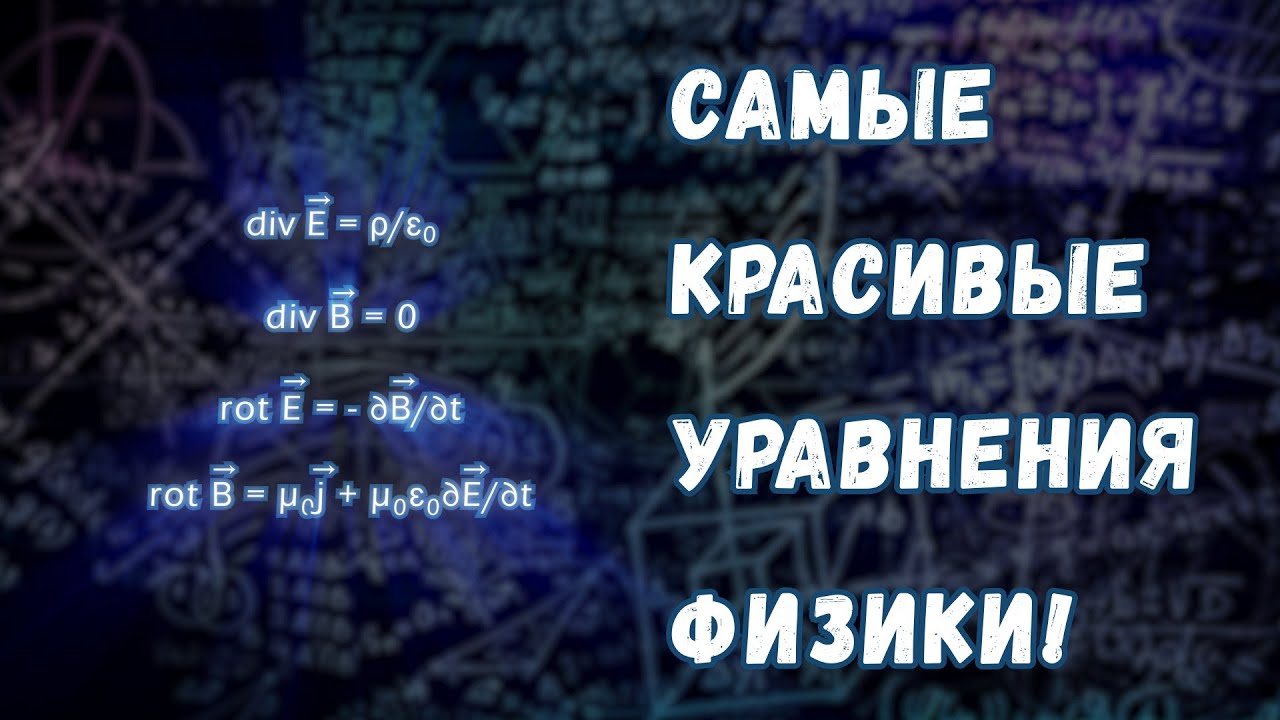
Real-world applications in physics, including Maxwell's equations in electromagnetism and the analysis of fluid dynamics (velocity fields, sources, and sinks).
288.7K views7Klikes15:36Original Release: 2019-09-18
Professor Dave again, let’s check out vector fields.
We spent a lot of time with vectors when we learned about linear algebra, and not surprisingly, we won’t be done with them any time soon.
We are used to vectors being made of components which are scalars, for example <2,1> which can also be written as 2i+1j.
We then got used to being able to move these vectors around however we wanted.
But now we are going to introduce vector fields, which can be thought of as functions that take in coordinates and give back vectors.
These vector fields will end up having vectors assigned to every point throughout the coordinate system, as shown here.
Of course, we are not limited to just two dimensions, vector fields can exist in any number of dimensions, and an example of a three dimensional field is shown here.
These vector fields can have a variety of practical interpretations, such as a force being exerted through space, or as the representation of motion.
But for now we will just focus on the general concept of a vector field and cover some basics.
As we mentioned, these vector fields can be thought of as functions, F of x and y, where the function has vector components that depend on the coordinates x and y.
The most general way we could express this is F(x,y) = P(x,y)i + Q(x,y)j, where P and Q are ordinary scalar functions that will depend on the coordinates x and y.
These scalar functions, also sometimes called scalar fields, determine the components of the vectors at each point in the coordinate system.
In three dimensions, our vector field could look like this.
F(x,y,z) = P(x,y,z)i + Q(x,y,z)j + R(x,y,z)k.
For a quick example, consider the vector field F(x,y) = -yi + xj.
To get an idea of how this vector field looks, let’s plug in a few coordinates and plot our resultant vectors.
We will take a few simple coordinates of the form (x,y) and plug them into the vector field.
To start, consider (1,0).
Here x = 1 and y = 0, so we get back the vector 0i + 1j, or <0,1>.
We will now plot this vector, originating from the coordinate we plugged in, (1,0).
We can quickly go through several more points and plot the resulting vectors as we go.
For (0,1) we get <-1,0>.
For (-1,0) we get <0,-1>.
For (0,-1) we get <1,0>.
For (1,1), <-1,1>.
For (-1,1), <-1,-1>.
For (-1,-1), <1,-1>.
And for (1,-1), we get <1,1>.
We are starting to see a clear circular pattern here.
If we continued with more points we would see this continue, and that vectors increase in size as we move away from the origin.
This is the general approach that can be used when wanting to see what a vector field looks like.
Obviously we can’t plot out the vectors at all the infinite points of the coordinate system, but we can see the general trend quite quickly.
Now let’s bring back the del operator we introduced in the previous tutorial regarding gradient.
Recall that del is a vector made of the differential operators <d/dx, d/dy> or if in three dimensions <d/dx, d/dy, d/dz>.
The gradient of some function f, del f, is itself a vector field with components being the partial derivatives of the function, so <df/dx, df/dy>.
To get more specific, if we have a vector field F, and it can be written as the gradient of a function f, the vector field is called a “conservative vector field” and the function f is called a “potential function” for the vector field F.
There are two more uses for the del operator with vector fields, and these involve the vector dot product and cross product.
We can take the del operator and dot it into a vector field F.
This is referred to as the “divergence” of F. Similarly, we can take del cross F, and this is referred to as the “curl” of F. Let’s take a closer look at what these expressions are.
Recall that we can write a vector field F in the form <P(x,y,z), Q(x,y,z), R(x,y,z)> so for now we’ll just focus on three dimensions, while P, Q, and R will be ordinary scalar functions that depend on x, y, and z.
While we can take the divergence in any number of dimensions, the curl can only be taken in three dimensions.
First let’s look at the divergence, del dot F. Recalling from a previous tutorial how the dot product works, we will simply find the product of the corresponding elements of the vectors, and then add those up.
So del dot F ends up giving us d/dx P + d/dy Q + d/dz R, which means we take the partial derivative of P with respect to x, plus the partial derivative of Q with respect to y, plus the partial derivative of R with respect to z.
So the divergence of a vector field will no longer be a vector field, rather it will be a scalar field.
Consider the vector field F = <(x^2)y, -x/y, xyz>.
To find the divergence we will take del dot this expression, which gives d/dx[(x^2)y] + d/dy(-x/y) + d/dz(xyz).
All of these derivatives follow the power rule that we already know, so we end up with 2xy + x/(y^2) + xy, which simplifies to 3xy + x/(y^2).
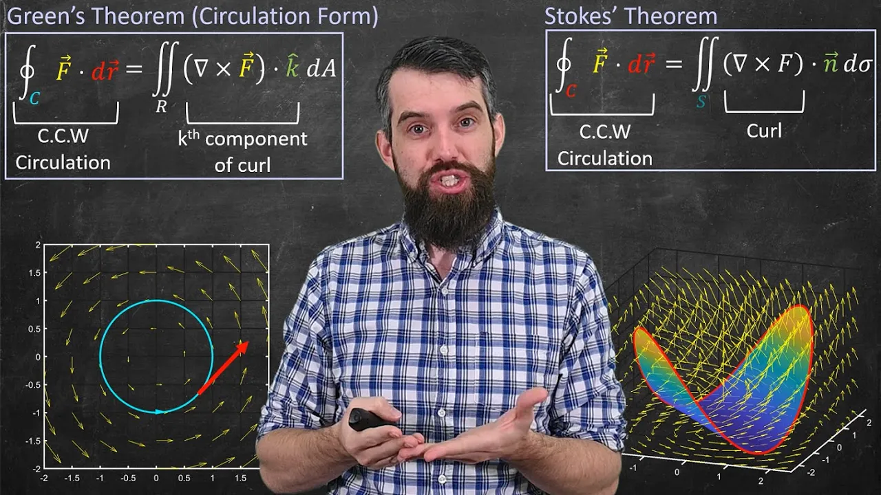
We will get more into the application of divergence in a future tutorial, but for now you can think of it as a measure of how much of the vector field is going out of some point.
Next let’s go over the curl.
As we mentioned, the curl will be the cross product between del and a vector field F.
Remembering how the cross product works from a previous tutorial, we set up a matrix with i, j, and k on the top row, the elements of del on the second row, and the elements of F on the last row.
Let’s once again consider the vector field F = <(x^2)y, -x/y, xyz>.
To find the curl we will take the determinant of the matrix i, j, k; d/dx, d/dy, d/dz; (x^2)y, -x/y, xyz.
Taking the determinant we get i times the quantity d/dy(xyz) - d/dz(-x/y), minus j times the quantity d/dx(xyz) - d/dz[(x^2)y], plus k times the quantity d/dx(-x/y) - d/dy[(x^2)y].
Now we take all these derivatives.
For the first term, this y becomes one so we get xz, and this expression has no variable, so it becomes zero.
For the second term, this x becomes one so we get yz, and again here there is no z so this becomes zero.
For the third term, this x becomes one, leaving us with negative one over y, and this y becomes one, leaving us with x^2.
Simplifying, we get xzi – yzj + (-1/y + x^2)k, or in vector form <xz, -yz, -1/y + x^2>.
This is the curl of our vector field.
Notice that the result is also a vector field.
So while the divergence gives a scalar field, the curl gives a vector field.
The curl represents the rotation of a vector field F, the direction of the curl being the axis of rotation and the magnitude of the curl being the magnitude of rotation.
Before we wrap up, let’s mention some interesting properties of divergence and curl.
First off, for a function that has continuous second-order partial derivatives, the curl of its gradient is always the zero vector.
This means that the curl of any conservative vector field is zero, because being conservative means the field can be written as the gradient of some function.
We can go ahead and show this by writing the gradient as <df/dx, df/dy, df/dz> and taking the curl.
To do this, we set up the matrix shown here and take the determinant.
We end up getting i times (d^2)f/dydz – (d^2)f/dzdy, minus j times (d^2)f/dxdz – (d^2)f/dzdx, plus k times (d^2)f/dxdy – (d^2)f/dydx.
This notation is how we express taking multiple derivatives of the function f, with the order of differentiation being the variables on the denominator from right to left.
If we took the derivative with respect to the same variable twice, say x, it would be expressed as (d^2)f/dx^2.
Now here’s where we need the continuous second derivative to come into play.
If these derivatives are all continuous, that means the order in which we take derivatives does not matter, meaning that (d^2)f/dydz is the same as (d^2)f/dzdy, and so on.
So all of these terms cancel and we are left with a vector that has a zero for all its components.
This is the zero vector and we have proved this property.
Another property is that if the components of F have continuous second-order partial derivatives, then the divergence of a curl is always zero.
We can prove this as well.
Jumping ahead and writing out the components of the curl, we get del cross F being equal to <dR/dy - dQ/dz, dP/dz - dR/dx, dQ/dx - dP/dy>.
Remembering what del represents and taking the dot product of del and this expression will result in the derivative of the first element with respect to x, plus the derivative of the second with respect to y, plus the derivative of the third with respect to z.
This gives us [(d^2)R/dxdy – (d^2)Q/dxdz)] + [(d^2)P/dydz – (d^2)R/dydx)] + [(d^2)Q/dzdx – (d^2)P/dzdy)].
Once again, if these are all continuous, the order of differentiation does not matter, and since this is all just one long series of terms being added and subtracted anyway, we can find the corresponding terms and get them all to cancel, giving us zero and therefore verifying the property.
Vector fields are a very useful concept, and being able to take the divergence and curl of these fields allows for a surprisingly wide variety of calculations.
There are several important theorems that utilize these operations, so let’s check out some of those next, but first, let’s check comprehension.
Up Next

21:02
Line Integrals Explained: Intuitive Multivariable Calculus Tutorial
@FoolishChemist
262.3K views•2024-08-19

4:43
Elliptic Curve Cryptography Explained: ECC, ECDSA, ECDH
@PracticalNetworking
28.5K views•2024-10-21
5:53
Divisibility, Prime Numbers, & Prime Factorization | Math Basics
@ProfessorDaveExplains
158.6K views•2017-08-20

6:00
The Mathematical Impossibility of Accurate World Maps
@Vox
23.3M views•2016-12-02
Related Study Plans & Knowledge Roadmaps
Structured learning paths in Mathematics
mathematics
Tensor Calculus: Vectors to Riemann Curvature
01Mathematical Foundations: Linear Algebra & Calculus
02Covectors, Dual Spaces, and Tensor Basics
03The Metric Tensor and Index Gymnastics
+ 2 more learning modules
40h5 modules
Explore Roadmap
mathematics
Gödel's Incompleteness: Logic, Proofs & Limits
01Introduction to Formal Systems & Hilbert's Dream
02Set Theory, Cardinality, and Cantor's Diagonal Argument
03Arithmetization and Gödel Numbering
+ 2 more learning modules
14h5 modules
Explore Roadmap
mathematics
Galois Theory: Fields, Groups & Solvability
01Foundations of Abstract Algebra: Groups & Fields
02Polynomials & Field Extensions
03Splitting Fields & Symmetries
+ 2 more learning modules
24h5 modules
Explore Roadmap
mathematics
Non-Euclidean Geometry: Models & Geodesics
01Euclid's Fifth Postulate and the Birth of New Geometries
02Hyperbolic Space and the Poincaré Disk Model
03Geodesics: Defining Straight Lines in Curved Spaces
+ 2 more learning modules
15h5 modules
Explore Roadmap