













![[초보] 음악 장르 분류 인공지능과 음악 추천 알고리즘 만들기](https://i.ytimg.com/vi_webp/IE6lue0qusQ/maxresdefault.webp)









This video demonstrates how to extract spectrograms from audio files using Python and the Librosa library, covering the complete workflow from loading audio files with librosa.load() to computing the Short-Time Fourier Transform (STFT) with librosa.stft(), converting the complex STFT output to a spectrogram via squared magnitude, and applying perceptual transformations using librosa.power_to_db() and log-frequency scaling to create log-amplitude spectrograms that better match human auditory perception; the practical demonstration compares spectrograms across different musical genres (classical, rock, jazz) to illustrate how spectrogram visualization reveals distinct characteristics of each genre.
Extract Audio Spectrograms with Python & Librosa
Added:Basic Python Programming & Data Science Stack: Familiarity with Python syntax, NumPy array manipulation, and Matplotlib for basic plotting and data visualization.
Fundamentals of Digital Audio: Understanding how sound is digitized, including concepts like sampling rate (Hertz), bit depth, channels, and time-domain waveforms.
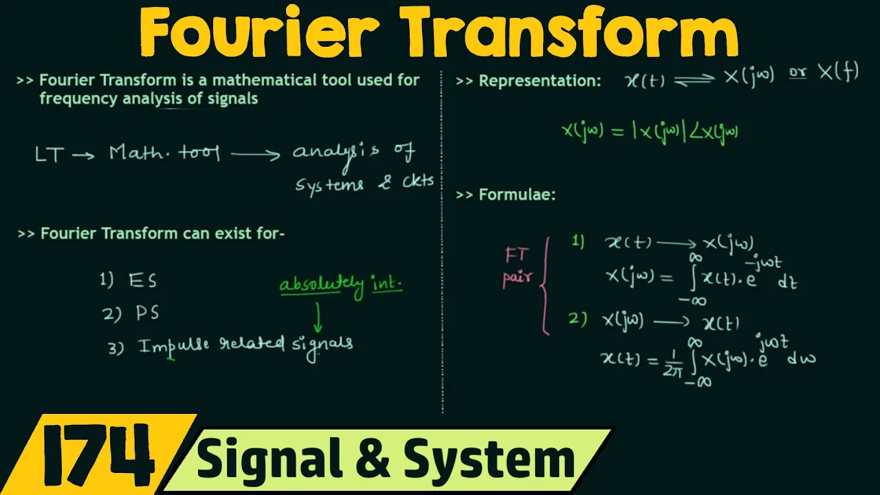
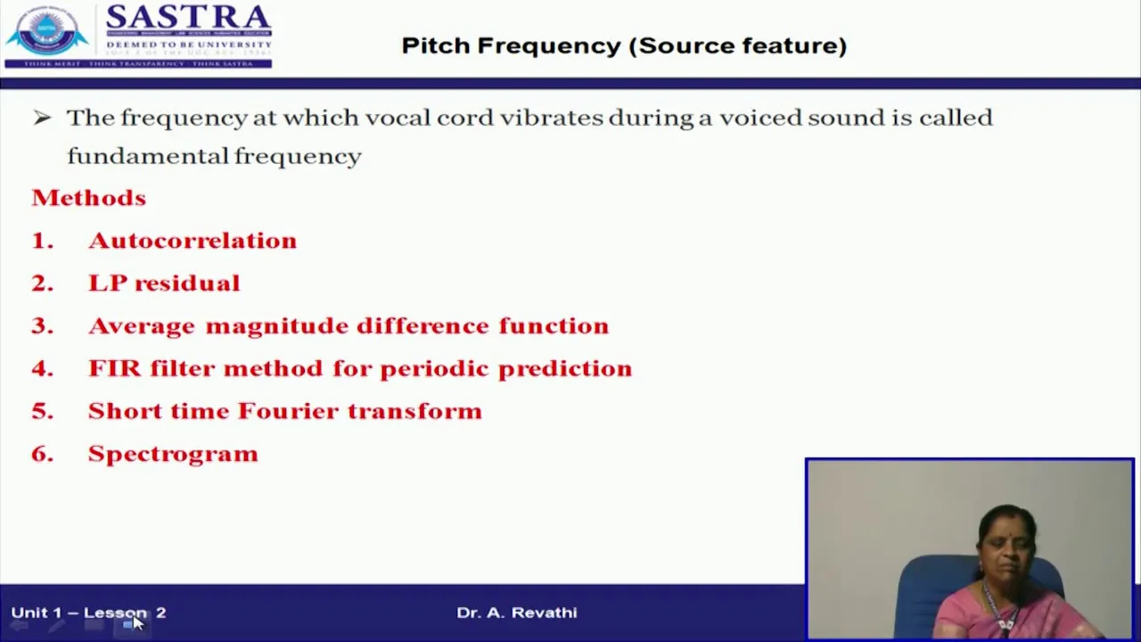
The Fourier Transform: A conceptual understanding of how time-domain signals are converted into the frequency domain, specifically the Short-Time Fourier Transform (STFT).
Logarithmic Scaling & Human Perception: Understanding how frequency and intensity are scaled logarithmically (e.g., decibels and the Mel scale) to align with human hearing.
Mel-Frequency Cepstral Coefficients (MFCCs) & Chroma Features: Moving beyond basic spectrograms to extract features optimized for speech recognition and musical harmony analysis.
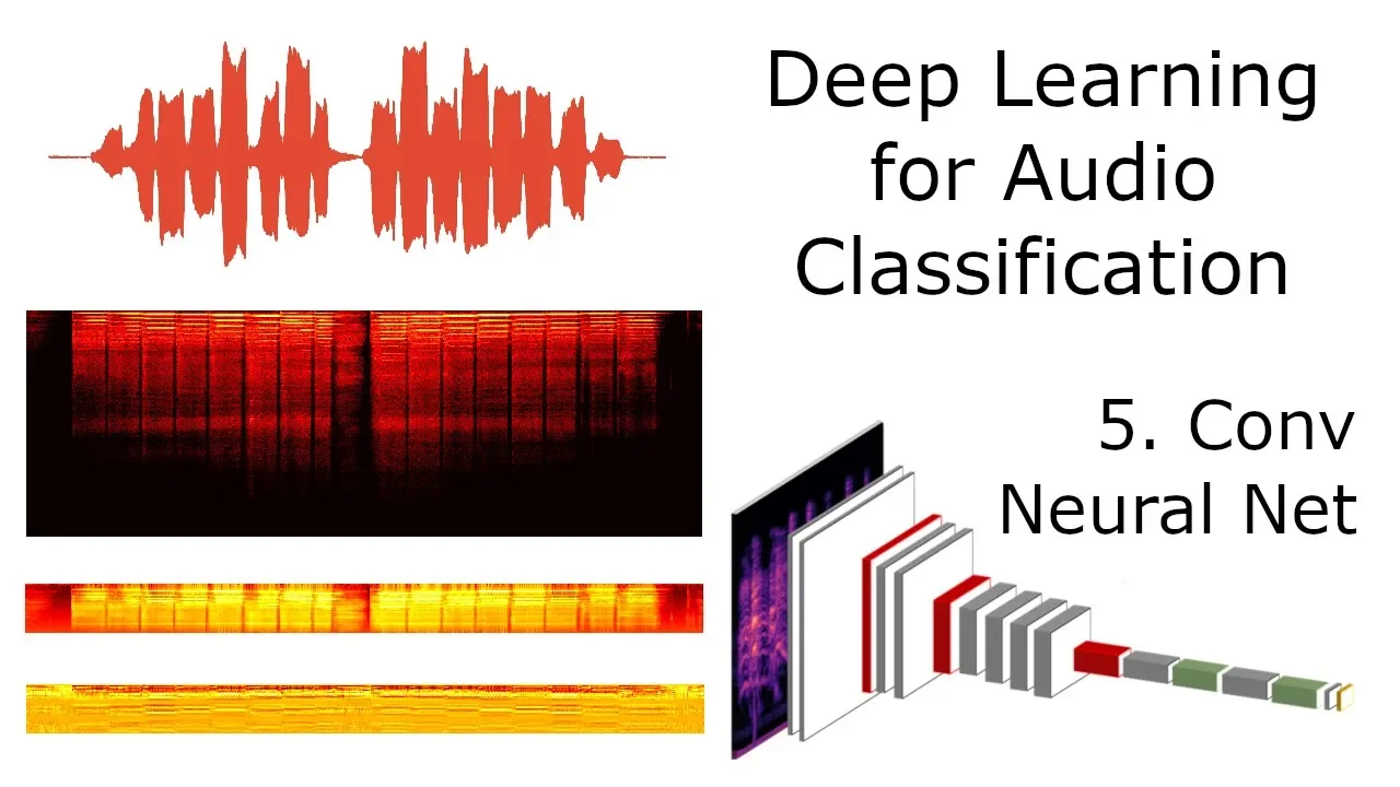
Deep Learning for Audio Classification: Utilizing 2D spectrograms as image inputs for Convolutional Neural Networks (CNNs) to perform music genre classification or sound event detection.
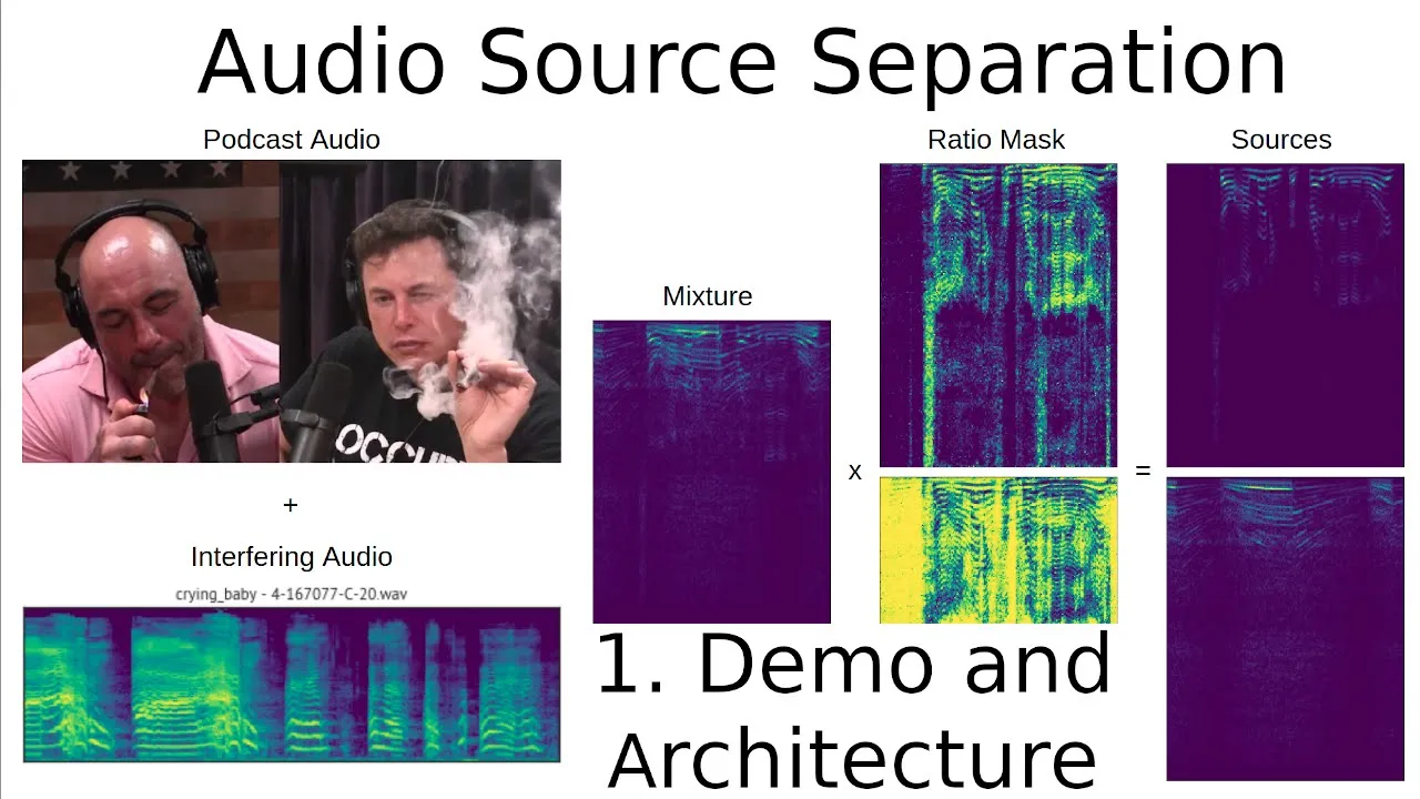
Audio Source Separation: Implementing algorithms to isolate vocals, drums, and other instruments from a single mixed audio track using toolkits like Spleeter or Librosa's decomposition tools.
Music Information Retrieval (MIR) Systems: Developing practical applications such as automatic beat tracking, onset detection, chord recognition, or audio fingerprinting.
78.4K views1.5Klikes23:25Original Release: 2020-09-10
Hi everybody and welcome to a new exciting video in the audio signal processing for machine learning series.
Last time we learned about a short time fiery transform and spectrograms in a theoretical way. This time it's time to actually use Python and the audio processing library to extract spectrograms from audio file.
So let's get started. So I already wrote a Jupyter notebook here and so I'm going to just like run through it and I'm going to tell you like what I'm doing and the different steps like to actually extract uh spectrograms. So the first thing that we want to do is just like import some uh like libraries. So we import OS so that we can uh load audio like our audio files. We'll import librosa librosa.isplay for uh just like showing visualizing like the spectrograms and we'll import like nonpie and map lib.pipplot for um actually doing or just like plotting uh the spectrograms like other results that we'll have. Okay. So let me import all of this and then we want to just like load audio files with librosa. So uh we are going to be working with four different audio files. So the first one is just like a scale and uh yeah it's just like resides like at this path.
Then we're going to have um kind of like a 30 second snippet from the BC 30 second snip snippets from Red Hot Chili Peppers and 30 second snippet from uh Duke Ellington. So we have like three different musical genres represented.
some classical music with the BC rock music with the red hot chili peppers and jazz with Juke Helington. Okay, but first thing let's try to listen to this music. So or and so we get like an idea what we're dealing with. And so here we go. So if you do I ipd.audio and you pass the uh the file then you're going to be able to directly listen to the uh to the audio files in a Jupyter notebook. By the way, this IPD comes from this import over here. So you just like important display as IPD and then you can use it. Okay. So now let's listen to like this different uh audio files. So the first one is going to be a scale uh played on a piano.
[Music] Okay. So, yeah, it's just repeated a couple of times. Then we have the music from Deusci, from the Red Hot Chili Peppers, and from Duke Ellington. So, let's listen.
If you guys followed along so far with the series, you probably already recognized this piece cuz we used it in a previous video.
So here you have like a huge crescendo, right, with all of this string instruments, right? You get the idea. So a very nice smooth uh like string driven uh orchestral piece. And then we have a song from the Red Hot Chili Pants.
Okay, you get the idea and probably you are also familiar with that song. Then moving on to this jazz piece from Jal by Jal.
[Music] Very smooth, right?
[Music] Okay, you get the idea. So what we'll do is try to extract the uh spectrogram from this and visualize them and compare them. Okay, so what we want to do first is just let you load the audio files with librosa. So we've done this multiple times in earlier videos. So uh what we do is just like librosa.load and we pass like the name of the or the path to the file. What we get back is a signal a numpy array and then we also get back the sample rate which when it's defaulted is going to be equal to 22,50 hertz. Okay. So let's move on to this next step. What we can do or what we should do is extract the short time fier transform. And this is very easy with librosa because we have a function that does that u super quickly. So the first thing we want to do is just let's set a couple of parameters. So we'll set the frame size equal to 24,48 hertz samples sorry and the hop size is going to be equal to 512 samples. Again these are quite typical parameters for like the frame size and the hop size. Uh if you don't know what I'm talking about I highly suggest you to go check out my previous video on the theory behind the short time for your transform. I'm just like taking for granted that you've watched that video or you are familiar with the short time for your transform.
So I'm not going to get into details what all of these parameters actually mean in this um video. Okay. So let's move on. Now uh I can extract the short time for transform using this uh function which is great uh librosa.st. And then I should pass in the signal.
And uh the first thing that we'll see here and the spectrograms that we'll analyze is are with regard with the with the scale just like to see how that is represented in a spectrogram and it's going to be easier to visualize than like all the other music that we've uh listened earlier. Then we should pass the frame size and we should pass it uh so with this keyword argument called n uh - fftft n fft and then we pass the hop uh length um keyword argument and we pass our hop size over here. Okay, so we do this and then now let's take a look at the shape of the short time for transform. So as we uh saw in the previous video, this is going to be like a b- dimensional array and specifically like the first dimension is relative to the the frequency. Uh and so here we have like um all the frequency bins and this these are equal so like this number is equal to half the frame size plus one. So it's basically 248 / 2 which is 1,24 + 1,025. Okay. So it checks out. Good.
And here uh like on the columns uh the second dimension of this matrix we have the um number of frames. It's basically like the temporal bins. And in this case we have like 342 temporal bins. And if you want to know how to get from uh like a signal to like a certain number of um frames just like to make that calculation I have like the formula in the previous uh video regarding short time fa transform. Okay. So now the next thing that we want to see is the actual type of the different items that we have in the uh short time for transform result or in the matrix. So here we just like take the item at uh col row 0 column 0 and as you can see the type is a complex number and this doesn't come as a surprise because the output of a short-time FIA transform is a series of like complex fier coefficients and so uh yeah so we expect that each of the items which is a FIA coefficient for a given uh like frequency bin and a given like frame is a complex Um but now what we want to do is actually calculate the spectrogram. So we need to to move from the short-term FIA transform to the spectrogram. So how do we do that? Well that's easily done because we just like take the squared magnitude of the short time for transform. So we just like use like this nunpy. Aabs absolute value and we pass in the um short time for a transform result here and then we square the result and this is going to be equal to the spectrogram. Okay. Yeah, not that.
Let me move on. Let's take a look at the shape here. And once again, not surprisingly, we have like this shape.
So 1,025 number of bins and 342 uh number of frames which is the same that we used to have like with the short-term FA transform results and that checks out because all we're doing is just like taking the magnitude the squared magnitude. So the the shape of the matrix uh of the original matrix doesn't change but what does change is the type of the items. In this case we have uh floats and this makes sense because we are taking like the the magnitude here and so basically we are moving from the complex number to like a real number and this is the spectrogram and this is like what we can actually visualize um uh on a heat map and so let's see how we can easily visualize the spectrogram uh with librosa and so here I wrote like a little function and here this is the signature. So you see uh y capital y is just like the um uh it's the spectrogram. Then I pass in the sample rate, the hop length and the y axis. And here like I'll default is let's say linear. We'll see what this means like in a second. But before let's just uh take a look at what I do here. I just like instantiate um a figure uh specifying like the the figure size here using like map lib. And then here comes the magic. We can use librosa.d display.spec show to uh visualize uh any type of spectrogram like um signals. And so here what uh like this function expects is y. So basically like the um spectrogram then the uh sample rate the hop length the x-axis which is going to be equal to time. So, we're going to have like on the x- axis we're going to have like time and on the y- axis we're going to have like a type of um representation that's linear and then I'm going to add a color bar here and you'll see what this does. It's basically like a legend that uh provides us information about like the uh how to map the colors into like the different like intensities like of the uh of the signal of the amplitude. Okay. So now let me run this and now we can plot the spectrogram and I'll pass in the uh spectrogram for like the scale scale like audio file. I'll pass in the sample rate and the hop size. And so let's see what happens here. And here we go our first visualization of a spectrogram.
But this doesn't look great, does it? So obviously like the idea here is that the the brighter the color and the more energy you have like in that uh frequency bin right and so we see a little bit of like activity down here and it's repeated and so probably you can guess that this is like the two scale like the fundamental uh frequencies of the scales and in indeed you see that these like tend to like run up uh and it's repeated twice because if you remember like in that audio file we the same scale repeated twice but still like everything is black so it means that it has like very very little energy. So why is that the case? Well, it turns out that this is how sounds like work. So uh but uh it's like the way we actually perceive like these energies and amplitude is not really linear as is the case like in this representation here but it it's actually logarithmic. And so uh to get like closer to the way we perceive a sound we need to do a kind of transformation of the uh intensities like of all the amplitudes here. And so we need to to move like all of this like amplitudes from the uh basically like linear representation to a logarithmic representation which is like more perceptually significant. we can easily move from a linear representation of amplitude to a logarithmic one using uh this uh handy function from librosa called power to db and db stands for decibb. Now if you are not familiar with deciBB I suggest you to go check out this video where I talk about decibb and introduce them and explain like how they work. But basically under the hood what happens is that decibb are actually applying some kind of like logarithmic transformation. So when you use this power to db you're moving like from the power representation like of the intensity like to uh decibb and so we do this and we get back a log amplitude uh spectrogram here. And so we can then just like plot that with our function.
So plot spectrogram instead of passing the actual like spectrogram of scale we pass the log amplitude spectrogram and again we pass the sample rate and the hop size. Okay. So if we do that we get this result which is way better like than the one that had we had before. So here we start to see like some uh energy like burst like of energy like down here. And as you can see here probably like this this is like constant uh like notes then you move up you move up up up up. So this probably is just like the fundamental frequencies for the scale that we played. And if you're wondering about like all of this other kind of like burst uh like of energies like at higher frequencies, those are uh the harmonic components of the original of the fundamental frequency for the scale.
Now we have like twice the same thing because if you uh remember like yeah we had twice the the scale like performed and so the same pattern is repeated uh twice. I I bet like they just like copy paste it like that the same scale like uh in the same in the audio file. Okay.
But here there's still something that's uh like a little bit weird which is like that on the frequency side uh I mean everything like is very squashed and then that the reason why is that the case is because like we are using some kind of like a linear frequency representation right but if you followed along with the series in one of like the initial videos that we had in the series I explained that the way we perceive uh frequency is logarithmic. It's not a linear. So what we want to do probably uh to have a representation of the spectrogram that's more kind of like in line uh with the way that we perceive um frequency is to actually apply some logarithmic transformation on the frequency as well as the amplitude. So how do we do that? Well, that's extremely simple uh with librosa. And so what we want to do is to create a log frequency log spectrogram uh um representation. And so what we do like in the function that I wrote you just like pass this uh keyword argument y-axis and you put it to log. But what this actually does under the hood is uh we are just like passing that in uh this like y-axis in the libresa.spec a spec show uh function and we pass it here. And so uh the default that we were using was like a y-axis is equal to linear. And in other words, we're using like a linear representation of the frequency. But if we put it equal to log, we're going to be using like a log representation of frequency. Okay. So now let's take a look at this and see how it looks like.
Okay, good. So as you can see here we have a uh log uh representation and now like this is like way more like spaced out and as you can see so this makes a lot of sense because like we start with a uh basically like the middle C or like C4 the the central C on the keyboard which is like this note here. Then we go up to a D. So we do a C, D, then up to E, F, G, A, B, and then back to C, but at the octave above. And so we can clearly see all of the scale going up here. And it has also like some slightly like different duration, like each note is played with a different duration. So I'll just like play you back like the the scale once again so you can notice that. Okay.
Okay.
And it's this, right?
D, right? Okay.
Uh, good. So, the next thing that I want to do is just like visualize all the other songs from Yeah. the different genres. So like the uh classical orchestral piece from uh Deucey, the red hot chili pepper like rock song and the jazz blood from uh Duke Ellington. Okay.
So I'll quickly go explain what I do here, but it's basically what what we've already done in a more extended way with the with the scale. uh but basically what I do here is I extract the short time 4A transform as a first thing and then uh I just uh get the u magnitude the square magnitude and then apply this power to decibb and then we get this signals for the busy for red dot and for duke and these are the log spectrograms for these different songs and then I just like pass those like into like this plot spectrogram function and I ask to have a log representation of the frequency and so what we're going to see is a log frequency log amplitude spectrogram. Okay, so let's take a look at this. Okay, so the first one is the spectrogram for the classical music piece. This is the red hot chili peppers one and this is like the jazz piece.
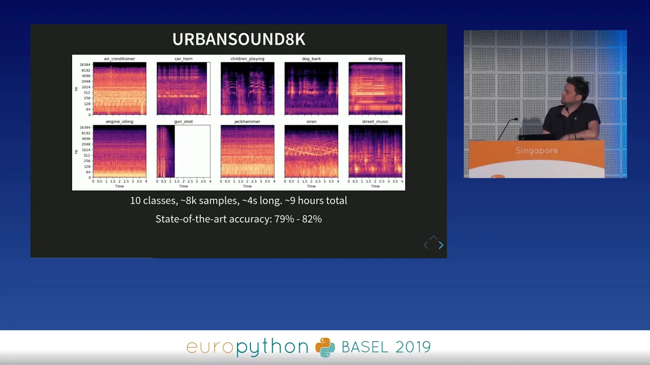
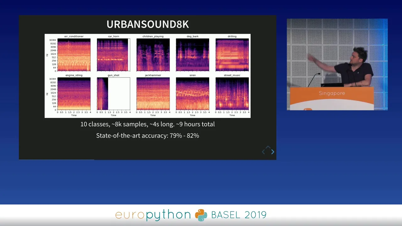
Okay, so is there any major difference that yeah we can see just like straight away? Yes, there is. So, in the case of classical music or this orchestral piece with a lot of like smooth string sounds, you see that the kind of like the distribution of the energy like in the different frequencies, it tends like to change right quite a lot. And obviously the redder uh in this spectrogram like the the uh the color and the more energy you have like in that frequency at that specific like moment in time, right? And uh so here as you see like if you remember we had like a huge crescendo a kind of like increase in intensity uh towards like the the center of like the the the snippet of that like the BC uh orchestral piece. And here you have it down here. So you have like higher frequency that get like kind of like higher energies like this. And then if you listen to the end of the piece, it tends to kind of like fade away. And you can kind of visualize that because like the this uh colors tends to like kind of like fade out. It's they're not as red as they used to be like in this central part for example. Now let's compare this kind of like smooth spectrogram to the red hot chil pepper one. Right. This is this feels like a way more kind of I I would say like like a pattern like that repeats itself like quite a lot and we have a lot of like activity in the lower uh like frequencies and this has also to do with the presence of uh like a kick drum. So you have like this bass um kind of like the the snare like with the with the with the bass drum uh kind of uh creating like this typical like rock pattern and you can see it here like in with the all of this activity here you have like a lot of repetition. So take a look for example this like patterns like here like in red like this. Okay. And so you see that with the rock piece you have like a lot of energy like in the lower um frequencies and you have like this patterns that you can kind of recognize and that's because the music is based off like patterns rhythmical as well as like melodic ones. Okay. And and then you have like the jazz piece uh by Jake Ellington. And here I could say that's a little bit like of the two worlds, right? So you still have like certain patterns that you can clearly see and that's because we we had like some kind of like basic like a groove with a drum kit and with bass um but uh still like it's kind of like more fluid, right?
It's not as strict as the rock uh piece by the red hot peppers, right? Okay. So here like at a glance you you can see that spectrograms can reveal a lot about different musical genres. Obviously like this is just like a an anecdotal uh example but more yeah more often than not these are like certain features that you actually see across different genres like when you like look at their spectrogram. So you can have like a a fair guess if you're experienced in uh visualizing spectrograms whether like you're dealing with a classical music kind of like piece or you're dealing with a a rock uh like valad or whatever.
That's all for today. I hope you enjoyed the video. Next time we're going to move on to another flavor of spectrograms called male spectrograms which are more psychological perceptually relevant than the royal spectrograms that we've seen here. So if you enjoyed the video and found it useful, please leave a like. If you haven't subscribed and you would like to see more videos like this, well just subscribe to the channel. And if you have any questions, as always, just like leave them in the comment section below. I hope I'll see you next time.
Cheers.
Up Next

9:24
Speech-to-Text with OpenAI Whisper in Python | Hugging Face
@1littlecoder
22.6K views•2022-10-11

12:54
Triumph of Orthodoxy Icon: Byzantine Art & History Explained
@BenCallan
2.1K views•2024-08-06

9:49
FastAPI vs Flask vs Django: Choosing the Right Python Web Framework
@TechWithTim
302.5K views•2024-05-26

1:42
Game of Thrones Opening Credits: A Cinematic Analysis
@gameofthrones
46.3M views•2011-04-18
Related Study Plans & Knowledge Roadmaps
Structured learning paths in General & Interdisciplinary Studies
general-studies
Elevator Engineering: History, Physics & Cities
01From Hoists to Safety Brakes: The Dawn of Vertical Lift
02Hydraulic vs. Traction: The Engineering Physics of Elevators
03Modern Speed, Safety, and Algorithms
+ 2 more learning modules
12h5 modules
Explore Roadmap
general-studies
Rubber: Material Science, History & Geopolitics
01Origins of Natural Rubber & Mesoamerican History
02The Chemistry of Natural Rubber & Vulcanization
03The Geopolitics of the Rubber Boom & Colonization
+ 2 more learning modules
12h5 modules
Explore Roadmap
general-studies
Containerization: Evolution, Logistics & Trade
01Ancient Trade & Bulk Cargo: Amphorae to Barrels
02The Industrial Revolution & Cardboard Packaging
03The Containerization Revolution: Malcom McLean
+ 2 more learning modules
12h5 modules
Explore Roadmap
general-studies
Textile Tech: Evolution, Labor & Global Impact
01Pre-Industrial Textiles: Handloom & Cottage Industry
02Mechanization: The Spinning Jenny to the Power Loom
03The Factory System & Global Labor Transformation
+ 2 more learning modules
10h5 modules
Explore Roadmap