For a bounded function f on [a,b], the lower Riemann integral is the supremum of all lower sums L(f,P) over partitions P, denoted by ∫ₐᵇ f(x)dx, while the upper Riemann integral is the infimum of all upper sums U(f,P), denoted by ∫ₐᵇ f(x)dx; a function is Riemann integrable if and only if these two integrals are equal.
Upper and Lower Riemann Integrals with Examples | Real Analysis
Added:Deep Dive
Understanding of bounded functions on closed and bounded intervals [a, b].

Funcții mărginite (aplicații) | Lectii-Virtuale.ro
7.3K
A function f defined on a set A with values in R is bounded if there exist real numbers a and b such that f(x) ∈ [a, b] for all x in A. For functions defined on closed intervals, boundedness can be proven by transforming the interval inequality. For linear functions f(x) = mx + c, multiply the interval bounds by m and adjust by c. For power functions f(x) = x^n, raise the interval bounds to the power n. For discrete functions, calculate all values and find the minimum and maximum.
Click to watch →

JEE: Continuity | JEE Live Sprint 2.0 | Unacademy JEE | JEE Maths | Nishant Vora
135.3K
A function is bounded if there exist real numbers m and M such that m ≤ f(x) ≤ M for all x in the domain. A continuous function defined on a closed interval is always bounded. This is because the Extreme Value Theorem guarantees that the function attains a minimum and maximum value on the interval.
Click to watch →

微分積分学⑧ ~ 連続関数の最大値の定理 ~
789
To prove a continuous function on a closed interval is bounded, define the set Σ = {x | a < x ≤ b and f is bounded on [a, x]}. This set is non-empty (continuity at a implies boundedness near a) and bounded above by b, so it has a supremum c. By contradiction, assume c < b. Since f is continuous at c, there exists δ > 0 such that f is bounded on [c-δ, c+δ]. Since c is the supremum of Σ, there exists d in Σ with c-δ < d < c. Since d is in Σ, f is bounded on [a, d]. Combining these, f is bounded on [a, c+δ], implying c+δ is in Σ, contradicting that c is the supremum. Thus c = b. Similarly, continuity at b implies boundedness near b, completing the proof that f is bounded on [a, b].
Click to watch →

تمرين شامل في المتتاليات
14.3K
To prove a function f is strictly increasing on its domain, calculate its derivative and show f'(x) > 0. For f(x) = (13x + 13)/(9x + 13)², f'(x) = 169/(9x + 13)² > 0 for all x ≥ 0. On a closed interval [a, b], a strictly increasing function satisfies f(a) ≤ f(x) ≤ f(b). For f on [0, 1/4], f(0) = 1/13 and f(1/4) = 260/3481, so 1/13 ≤ f(x) ≤ 260/3481 for all x in [0, 1/4].
Click to watch →

Advanced calculus, continuity 3
170
A function is bounded on an interval if there exist real numbers M and m such that m ≤ f(x) ≤ M for all x in the interval. M is called an upper bound and m is called a lower bound. The formal definition states that a function f is bounded on a set S if there exists a real number M such that |f(x)| ≤ M for all x in S. A function is continuous on a closed interval [a, b] if it is continuous at every point in the interval, meaning for any point c in [a, b], the limit of f(x) as x approaches c equals f(c). These concepts are fundamental in real analysis and form the basis for understanding function behavior.
Click to watch →
Deep Dive
Concepts of Supremum (Least Upper Bound) and Infimum (Greatest Lower Bound) of a set of real numbers.

Topology Of Real Numbers Chapter1 Sequence And Series Math |For B.Sc 4th Sem 2nd Year Basic Concepts
51.6K
The supremum (sup) is the least upper bound of a set - the smallest number that is greater than or equal to all elements. The infimum (inf) is the greatest lower bound - the largest number that is less than or equal to all elements. For any non-empty set of real numbers that is bounded above, a supremum exists. Similarly, for any non-empty set bounded below, an infimum exists. For example, in the set {1, 2, 3, 4, 5}, the supremum is 5 and the infimum is 1.
Click to watch →
Apa itu Supremum dan Infimum?
28.3K
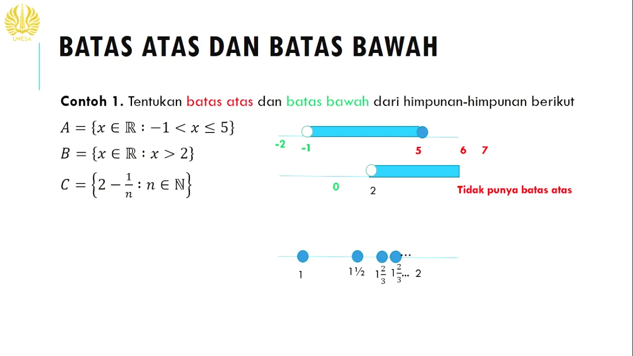
The supremum (least upper bound) of a set is the smallest number that is greater than or equal to all elements in the set. The infimum (greatest lower bound) is the largest number that is less than or equal to all elements. For set A = (-1/2, 5], supremum is 5 and infimum is -1/2. For set B = (2, ∞), there is no supremum but infimum is 2. For set C = {2 - 1/n | n ∈ ℕ}, supremum is 2 and infimum is 1. These concepts are fundamental to real analysis and help describe the precise boundaries of sets.
Click to watch →

Least Upper Bound & Greatest Lower Bound | Supremum & Infimum | Real Analysis
440
In Real Analysis, the Least Upper Bound (Supremum) and Greatest Lower Bound (Infimum) are fundamental concepts that guarantee the existence of bounds for bounded sets of real numbers. A set has a least upper bound if it is non-empty, a subset of real numbers, and bounded above; the least upper bound is the smallest real number that is greater than or equal to all elements in the set. Similarly, a set has a greatest lower bound if it is non-empty, a subset of real numbers, and bounded below; the greatest lower bound is the largest real number that is less than or equal to all elements in the set. The Completeness Axiom of real numbers ensures that these bounds always exist for bounded sets, a property that does not hold for rational numbers.
Click to watch →

Real analysis (lower bound and infiamum) part 3
8.2K
The greatest lower bound (infimum) is the largest lower bound of a set, and the least upper bound (supremum) is the smallest upper bound. Both are unique for any set. For S = {0, 1, 2, 3, 4}, infimum is 0 and supremum is 4. For S = {-1, -2, -3, ...}, no infimum exists. These concepts are fundamental to real analysis.
Click to watch →
Cotas, Supremo e Ínfimo #ConstruçãoDosNúmerosReais Aula09 - Professor Eduardo Garcez
8.7K
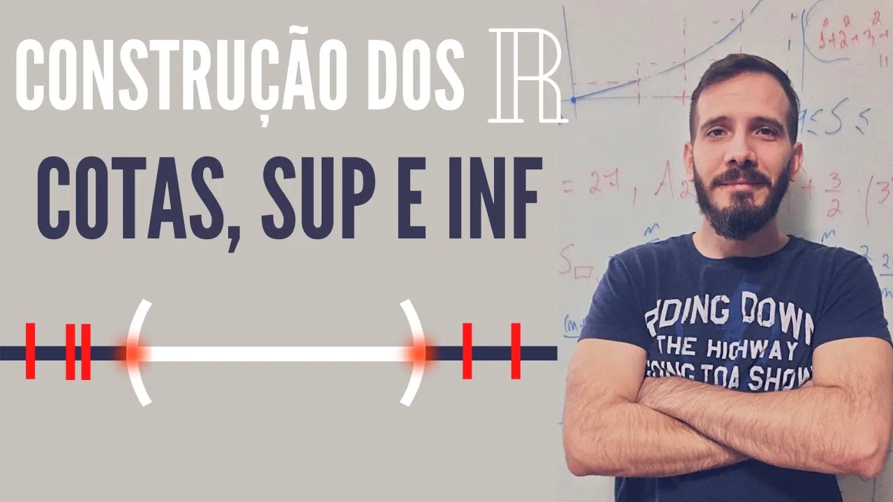
The supremum (supremo) is the least upper bound: a number s that is an upper bound AND any smaller number is not an upper bound. The infimum (ínfimo) is the greatest lower bound: a number i that is a lower bound AND any larger number is not a lower bound. For the open interval (0,1), sup = 1 and inf = 0, even though 0 and 1 are not in the set. These concepts are essential for understanding the completeness of real numbers.
Click to watch →
Deep Dive
The definition of a partition of an interval, including subintervals and partition norm/mesh.

Riemann stieltjes integral /L 4/ in real analysis bsc Msc csir net maths upsc maths gate maths
8K
A partition of an interval [a, b] is a finite set of points that divide the interval into smaller subintervals. For example, if we have the interval [a, b], a partition P consists of points a = x₀ < x₁ < x₂ < ... < xₙ = b. These points divide the original interval into n subintervals [xᵢ₋₁, xᵢ] for i = 1, 2, ..., n. The norm of a partition (||P|| or λ(P)) is defined as the maximum length of the subintervals created by the partition. If the subintervals have lengths Δx₁, Δx₂, ..., Δxₙ, then the norm is ||P|| = max(Δx₁, Δx₂, ..., Δxₙ). The norm measures how fine the partition is.
Click to watch →

CHAPITRE 1: Intégrale de Riemann
362
A partition (difivision) of an interval [a,b] is a finite set of points a = x₀ < x₁ < ... < xₙ = b that divide the interval into subintervals. The mesh (norme) of a partition is the maximum length of its subintervals: ||P|| = max(xᵢ₊₁ - xᵢ). A partition is uniform (équidistant) if all subintervals have equal length.
Click to watch →
Lec 21: Riemann Integral Part 2 | Real Analysis | UPSC Maths Optional By Sujit Shukla
379
A partition P of [a, b] is a finite set of points a = x₀ < x₁ < ... < xₙ = b. The mesh (norm) is the maximum subinterval length Δxᵢ = xᵢ - xᵢ₋₁. For uniform partition, Δxᵢ = (b - a)/n. The partition points are xᵢ = a + i(b - a)/n for i = 0, 1, ..., n.
Click to watch →

Riemann Integral | Definition of Partition , Norm , Refinement | #1 | New Era Maths Classes | Sem 5
37.2K
A partition of an interval [a, b] is a finite set of points x₀, x₁, ..., xₙ such that a = x₀ < x₁ < ... < xₙ = b, dividing the interval into n subintervals; the norm (or mesh) of a partition is the maximum length of these subintervals, denoted as ||P|| = max{xᵢ - xᵢ₋₁}; a refinement of a partition P is another partition Q that contains all the points of P plus at least one additional point, making Q a 'finer' partition than P.
Click to watch →

BSc 1st Semester Mathematics Integral Calculus | The Riemann Sums | BSc 1st Semester Maths Unit-5th
3.3K
Subintervals are consecutive pairs of partition points: Iᵣ = [xᵣ₋₁, xᵣ] for r = 1, 2, ..., n. The length of each subinterval is Δxᵣ = xᵣ - xᵣ₋₁. The norm of the partition, denoted ||P||, is the maximum length among all subintervals: ||P|| = max{Δxᵣ : r = 1, 2, ..., n}. The norm measures how fine or coarse the partition is.
Click to watch →
Deep Dive
The construction and calculation of Upper and Lower Darboux Sums for a given partition.

L2 | BSc1st Semester Mathematics Integral Calculus| Unit 5 l Riemann integral
493
A partition of a closed interval [a, b] is a finite set of points P = {a = x₀, x₁, ..., xₙ = b} where a < x₁ < ... < xₙ = b. Subintervals are [x₀, x₁], [x₁, x₂], ..., [xₙ₋₁, xₙ], with length Δxᵢ = xᵢ₊₁ - xᵢ. For a bounded function f on [a, b], the Darboux sums are: Lower Darboux sum L(P, f) = Σᵢ₌₁ⁿ mᵢΔxᵢ where mᵢ = inf{f(x) | x ∈ [xᵢ, xᵢ₊₁]}, and Upper Darboux sum U(P, f) = Σᵢ₌₁ⁿ MᵢΔxᵢ where Mᵢ = sup{f(x) | x ∈ [xᵢ, xᵢ₊₁]}. To calculate: identify partition points, find min/max values in each subinterval, calculate lengths, then apply the formula. Example: For f(x) = x on [0, 4] with partition {0, 3, 4}, L(P, f) = 0×3 + 3×1 = 3 and U(P, f) = 3×3 + 4×1 = 13.
Click to watch →

Integration theory of Riemann-I
21.4K
For a bounded function f on [a,b] and a partition P, the upper Darboux sum U(f,P) is ∑Mᵢ(xᵢ-xᵢ₋₁) where Mᵢ = sup{f(x):x∈[xᵢ₋₁,xᵢ]}, and the lower Darboux sum L(f,P) is ∑mᵢ(xᵢ-xᵢ₋₁) where mᵢ = inf{f(x):x∈[xᵢ₋₁,xᵢ]}. These sums provide upper and lower bounds on the area under the curve. Key properties include: L(f,P) ≤ U(f,P) always, and refining a partition (adding more points) increases the lower sum and decreases the upper sum.
Click to watch →

BSC 3RD SEMESTER|| MGSU|| UNIT-3|| RIEMANN INTEGRAL|| EXAMPLES ||MANOJ SIR
269
This segment demonstrates the complete calculation of upper and lower Darboux sums. For the upper sum: on [0, 1], integrate f(x) = x + x² to get 5/6; on [1, 2], integrate g(x) = x² + x³ to get 73/12; total upper sum = 83/12. For the lower sum: on [0, 1], integrate g(x) = x² + x³ to get 7/12; on [1, 2], integrate f(x) = x + x² to get 23/6; total lower sum = 53/12. The instructor emphasizes that the upper sum uses the maximum function on each subinterval, while the lower sum uses the minimum function.
Click to watch →

Riemann Integration | IIT JAM/CUET PG 2026 | IIT JAM Mathematics |IIT JAM Score Booster
3.2K
The Lower Darboux Sum (LPF) is calculated by taking the infimum of the function on each subinterval, multiplying by the subinterval length, and summing all products. The Upper Darboux Sum (UPF) is calculated by taking the supremum on each subinterval, multiplying by length, and summing. LPF = Σ (infimum on subinterval j) × (length of subinterval j), UPF = Σ (supremum on subinterval j) × (length of subinterval j).
Click to watch →

ENDGAME II BSC FIRST SEMESTER MATHEMATICS II MJPRU/GJU/MSU/LU ALL STATE UNIVERSITIES II #bsc
3.4K
This segment covers Darboux sums, fundamental concepts in real analysis. The Upper Darboux Sum (UPF) is defined as ∑ᵢ₌₁ⁿ Mᵢ Δxᵢ, where Mᵢ is the supremum of f(x) on the i-th subinterval and Δxᵢ is the subinterval width. The Lower Darboux Sum (LPF) is ∑ᵢ₌₁ⁿ mᵢ Δxᵢ, where mᵢ is the infimum. For f(x) = x on [0,3] with partition 0, 1, 2, 3: M₁ = 1, M₂ = 2, M₃ = 3, so UPF = 1×1 + 2×1 + 3×1 = 6. Similarly, m₁ = 0, m₂ = 1, m₃ = 2, so LPF = 0×1 + 1×1 + 2×1 = 3. The instructor emphasizes that when all subinterval widths are equal, calculations simplify significantly.
Click to watch →
Prerequisite Knowledge
- Concept 01Understanding of bounded functions on closed and bounded intervals [a, b].
- Concept 02Concepts of Supremum (Least Upper Bound) and Infimum (Greatest Lower Bound) of a set of real numbers.
- Concept 03The definition of a partition of an interval, including subintervals and partition norm/mesh.
- Concept 04The construction and calculation of Upper and Lower Darboux Sums for a given partition.
Subsequent Learning
- Step 01The formal definition of Riemann Integrability (proving when the upper and lower Riemann integrals are equal).
- Step 02Riemann's Criterion for integrability and its application to specific function classes.
- Step 03The Fundamental Theorem of Calculus, bridging the gap between differentiation and Riemann integration.
- Step 04The classification of integrable functions (e.g., continuous functions, monotonic functions, and functions with finitely many discontinuities).
- Step 05Transitioning to Lebesgue Integration to handle highly discontinuous functions where Riemann integration fails.
Course Intro
Integral Defs
Integrability
Partition Sums
Sum Components
Limit Forms
Riemann Sums
Result Derive
Final Limit
Course Intro
0:02Playing Section
- 1
Covers engineering math topics like algebra and complex analysis.
- 2
Starts explaining real-valued bounded functions on a closed interval.
Lebesgue Integration
While Riemann integration (relying on upper and lower Darboux sums) is foundational, it has major limitations in advanced mathematical analysis. It struggles with highly discontinuous functions—for example, the Dirichlet function (which is 1 on rationals and 0 on irrationals) is not Riemann integrable. Lebesgue integration overcomes this by partitioning the function's range rather than its domain, utilizing measure theory to define the integral. This alternative framework allows a much broader class of functions to be integrated. Additionally, Lebesgue integration provides powerful convergence theorems (like the Monotone and Dominated Convergence Theorems) that allow the interchange of limits and integrals under much weaker conditions than the strict uniform convergence required by Riemann integration, making it the standard in modern analysis and probability.
Deep Dive
The formal definition of Riemann Integrability (proving when the upper and lower Riemann integrals are equal).

Lec-01 Riemann Integral. Upper and Lower Riemann Sums. Real II. Rudin (Urdu/Hindi)
7.9K
The Riemann integral is defined through upper and lower sums: for a bounded function f on [a,b], a partition P = {x₀, x₁, ..., xₙ} divides the interval into subintervals, where Mᵢ = sup{f(x) | x ∈ [xᵢ₋₁, xᵢ]} and mᵢ = inf{f(x) | x ∈ [xᵢ₋₁, xᵢ]}; the upper Riemann sum U(P,f) = ΣMᵢΔxᵢ and lower Riemann sum L(P,f) = ΣmᵢΔxᵢ; the upper Riemann integral is the infimum of all upper sums over all partitions, and the lower Riemann integral is the supremum of all lower sums; a function is Riemann integrable if and only if these two integrals are equal.
Click to watch →

Lec 05:Riemann sum, Equivalence of riemann integrability and darboux integrability: In hindi
7.9K
This segment presents the complete proof that Darboux and Riemann integrability are equivalent. The proof strategy involves showing that if a function is Darboux integrable (lower and upper Darboux integrals are equal), then it is also Riemann integrable. By combining the inequalities for lower and upper sums with the convergence of Riemann sums, the instructor demonstrates that the lower sum is less than or equal to the Riemann sum, which is less than or equal to the upper sum. As the partition mesh approaches zero, both lower and upper sums converge to the same value, which equals the Riemann sum limit. This convergence is guaranteed by the definition of Riemann integrability. The proof establishes that a function is Darboux integrable if and only if it is Riemann integrable, and both definitions yield the same integral value.
Click to watch →

تحليل رياضيء-الفصل السابع_مفهوم ريمان للتكامل(تكامل ريمان)_Def. of Riemann Integral/محاضرة { 68 }
15.1K
The Riemann integral is defined through upper and lower sums: for a bounded function f on [a,b] and partition P = {x₀, x₁, ..., xₙ}, the upper sum U(f,P) = Σᵢ₌₁ⁿ MᵢΔxᵢ where Mᵢ = sup{f(x) : x ∈ [xᵢ₋₁, xᵢ]}, and the lower sum L(f,P) = Σᵢ₌₁ⁿ mᵢΔxᵢ where mᵢ = inf{f(x) : x ∈ [xᵢ₋₁, xᵢ]}. The upper Darboux integral is U(f) = inf{U(f,P) : P is a partition}, and the lower Darboux integral is L(f) = sup{L(f,P) : P is a partition}. A bounded function f is Riemann integrable if and only if U(f) = L(f), in which case the common value is the Riemann integral ∫ₐᵇ f(x)dx. Unlike Cauchy integration which requires continuity, Riemann integration can handle functions with discontinuities by partitioning around discontinuity points.
Click to watch →

B.Sc 1st year Maths || Ch- The Riemann integral || 1-sem(2nd book)✍️✍️
21.3K
The Lower Riemann Integral is defined as the supremum of all lower sums (infimum of function values on each subinterval multiplied by subinterval width), while the Upper Riemann Integral is the infimum of all upper sums (supremum of function values on each subinterval multiplied by subinterval width). A function is Riemann integrable if and only if its Lower and Upper Riemann Integrals are equal. For a bounded function f on [a,b], if f is non-negative, the Lower Integral equals the Upper Integral if and only if f is Riemann integrable; if f is non-positive, the relationship reverses. The function must be bounded on the closed interval [a,b] and have no infinite discontinuities for the Riemann integral to exist.
Click to watch →

Real Analysis & Group Theory | IIT JAM Mathematics 2026 | Most Probable Questions | Lec 7 | IFAS
667
For a Riemann integrable function f on [a,b], the upper sum U(f,P) and lower sum L(f,P) converge to the same value as the partition norm approaches zero. For f(x) = sin(x) on [0,t], the integral is -cos(t) + cos(0) = 1 - cos(t). The upper and lower sums both approach this value. This is the definition of Riemann integrability.
Click to watch →
Deep Dive
Riemann's Criterion for integrability and its application to specific function classes.

PYQs on Riemann Integration | Short Cut tricks | CSIR NET & GATE 2011 to 2023
46.3K
A function is Riemann integrable on [a,b] if it satisfies any of these conditions: (1) Continuous on [a,b]; (2) Monotonic (increasing or decreasing) on [a,b]; (3) Has finitely many discontinuities; (4) Is bounded with countably many discontinuities and finite limit points; (5) Is of bounded variation. The converse is not true - integrable functions need not be continuous or monotonic. Uncountable discontinuities (like the Dirichlet function) always imply non-integrability. For discontinuous functions, Riemann integrability requires boundedness, countable discontinuities, and finite limit points. Functions with infinitely many discontinuities can still be integrable if they accumulate at a finite point.
Click to watch →

Integrabilidad Riemann - Teoría y ejercicios resueltos | Funciones de una Variable II | UNED
7.5K
Several classes of functions are guaranteed to be Riemann integrable: (1) Continuous functions on closed intervals; (2) Monotonic functions (non-decreasing or non-increasing) on closed intervals; (3) Functions with finitely many discontinuities. These conditions provide sufficient criteria for integrability without needing to verify the definition directly.
Click to watch →
![[s2 | 2025] Математический анализ, К. В. Правдин, лекция 26](https://i.ytimg.com/vi/0nwjqd7GkVI/maxresdefault.jpg)
[s2 | 2025] Математический анализ, К. В. Правдин, лекция 26
127
A function f is Riemann integrable on a closed interval [a, b] if and only if the difference between the upper Darboux sum and the lower Darboux sum approaches zero as the mesh (maximum subinterval length) of the partition approaches zero. This criterion provides a practical test for integrability without computing Riemann sums directly, as it only requires verifying that the oscillation of the function on each subinterval, weighted by subinterval length, becomes arbitrarily small for sufficiently fine partitions.
Click to watch →

Fonctions Riemann-intégrables : l'indispensable KIT de SURVIE !
19.1K
A bounded function f on [a, b] is Riemann-integrable if and only if the upper integral (supremum of integrals of all step functions greater than or equal to f) equals the lower integral (infimum of integrals of all step functions less than or equal to f). This means that when we take the supremum of all lower sums and the infimum of all upper sums, they converge to the same real number, which becomes the definite integral of f over [a, b].
Click to watch →

Бутузов В.Ф. - Математический анализ. Часть 1 - 15. Интегралы, ч.4. Свойства определенного интеграла
12.7K
A bounded function on [a, b] is Riemann integrable if and only if for any ε > 0, there exists a partition where the difference between upper and lower sums is less than ε. This criterion proves integrability of continuous functions and a broad class of discontinuous functions. Functions with infinitely many discontinuities can still be integrable if all discontinuities can be covered by finitely many intervals with arbitrarily small total length. Monotone functions are always integrable on any segment. Piecewise continuous functions (finite discontinuities of first kind) are also integrable. The Lebesgue integral generalizes Riemann integration to handle more complex functions.
Click to watch →
Deep Dive
The Fundamental Theorem of Calculus, bridging the gap between differentiation and Riemann integration.

Fundamental Theorem of Calculus (in Riemann Style)
857
The Fundamental Theorem of Calculus states that if f is continuous on [a,b], then the function F(x) = ∫ₐˣ f(t)dt is differentiable and F'(x) = f(x); more generally, if f is Riemann integrable on [a,b] and f(x) = g'(x) for some function g, then ∫ₐᵇ f(x)dx = g(b) - g(a). This theorem connects differentiation and integration, showing that the definite integral of a function equals the difference in values of its antiderivative at the endpoints. The proof uses the Mean Value Theorem and Darboux sums, demonstrating that integrability (not continuity) is the essential condition for this result.
Click to watch →

Lecture 03: Riemann integration and periodic functions
692
The Fundamental Theorem of Calculus connects Riemann integration with differentiation. Part 1: If f is continuous on [a,b] and F is an antiderivative (F' = f), then ∫ₐᵇf(x)dx = F(b) - F(a). Part 2: If f is differentiable and f' is Riemann integrable, then ∫ₐᵇf'(x)dx = f(b) - f(a). This theorem shows that Riemann integration is equivalent to the anti-derivative concept from high school calculus.
Click to watch →

Give Me An Hour And I'll Teach You Intro Analysis
11.7K
The Riemann integral is defined through upper and lower sums: for any partition, compute lower sum using infima and upper sum using suprema. A function is integrable if the supremum of lower sums equals the infimum of upper sums. Continuity on [a,b] guarantees integrability. The Fundamental Theorem of Calculus establishes that differentiation and integration are inverse operations: Part 1 shows that the integral function G(x)=∫ₐˣ f(t)dt is differentiable with G’(x)=f(x); Part 2 shows that if F is any antiderivative of f, then ∫ₐᵇ f(x)dx = F(b)-F(a).
Click to watch →

Riemann integral/L 8/ fundamental theorem in riemann integration bsc maths msc maths in hindi
19.1K
The Fundamental Theorem of Calculus establishes that differentiation and integration are inverse processes: if f(x) is continuous on [a,b] and F(x) is an antiderivative of f(x) (meaning F'(x) = f(x)), then the definite integral ∫_a^b f(x) dx equals F(b) - F(a). This theorem simplifies integration by allowing us to find antiderivatives and evaluate definite integrals through the difference of function values at the limits, rather than using the original definition of integration.
Click to watch →

MATA35 - Lecture 1b - Riemann sums and fundamental theorem of integral calculus
268
The Fundamental Theorem of Calculus establishes that differentiation and integration are inverse processes. Part 1 states that if f is continuous on [a,b], then d/dx [∫ₐˣ f(t) dt] = f(x), meaning the derivative of the definite integral from a constant lower limit to a variable upper limit x yields the original function f(x). Part 2 states that if F is any antiderivative of f (F' = f), then ∫ₐᵇ f(x) dx = F(b) - F(a). This allows computation of definite integrals without Riemann sums by finding an antiderivative and evaluating at bounds. The theorem connects the geometric interpretation of area with the algebraic process of antidifferentiation.
Click to watch →
Deep Dive
The classification of integrable functions (e.g., continuous functions, monotonic functions, and functions with finitely many discontinuities).
Садовничая И.В. | Лекция 31 по Математическому анализу, 2024, весна| ВМК МГУ
908
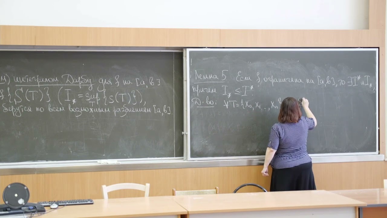
This section classifies important categories of Riemann integrable functions. The instructor proves that every continuous function on a closed interval is integrable, using the theorem of uniform continuity: for any ε > 0, there exists δ > 0 such that any partition with diameter less than δ makes the difference between upper and lower sums less than ε. The oscillation of a continuous function on each subinterval can be made arbitrarily small. The instructor also proves that every monotone function on a closed interval is integrable, since monotone functions are automatically bounded and their oscillation on each subinterval is bounded by the total variation (difference between endpoint values). These results establish that continuous and monotone functions form important classes of integrable functions.
Click to watch →

Фомичев В.В. | Лекция 26 по Математическому анализу, весна, 2025 | ВМК МГУ
326
This section extends the class of integrable functions to include monotone functions and functions with finite discontinuities. First, it proves that monotone functions on closed intervals are integrable: since monotone functions are bounded, and for any ε > 0, one can choose a partition with diameter less than ε divided by the difference between the supremum and infimum of the function, the difference between upper and lower Darboux sums will be less than ε. Second, it proves that functions with only a finite number of points of discontinuity are integrable: for a finite set of discontinuities, one can always construct a finite covering with arbitrarily small total length, satisfying Lebesgue's criterion. This extends integrability beyond continuous functions to include functions with jump discontinuities at finitely many points.
Click to watch →
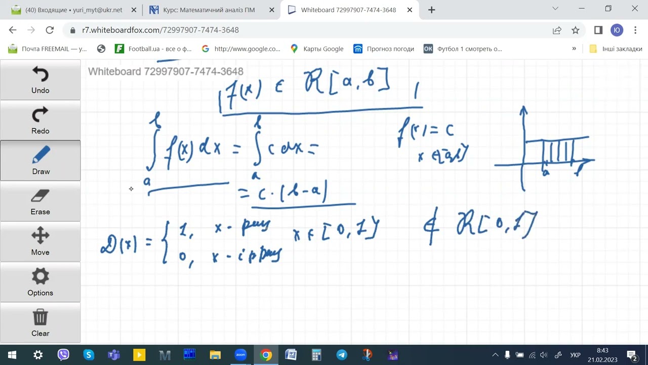
МА 2023 02 21 08 36 32 Юрій Митник's Лекція 18 Властивості визначен інтеграла Теорема Ньютона Лейб
148
Functions that are guaranteed to be Riemann integrable include: (1) Continuous functions on [a,b], (2) Monotonic functions (either non-decreasing or non-increasing) on [a,b], (3) Functions with a finite number of discontinuities on [a,b]. The Dirichlet function (1 at rational points, 0 at irrational points) is not integrable. The integrability of a function depends on its behavior and the nature of its discontinuities.
Click to watch →

Критерии интегрируемости. Классы интегрируемых функций. 2 семестр, 2 лекция
1.7K
Several classes of functions are guaranteed to be Riemann integrable: (1) Continuous functions on [a,b] are integrable because uniform continuity ensures that for any ε > 0, there exists δ > 0 such that |x - y| < δ implies |f(x) - f(y)| < ε/(b-a), making the difference between upper and lower sums less than ε. (2) Monotonic functions on [a,b] are integrable because for a non-decreasing function, the difference between upper and lower sums equals f(b) - f(a), which can be made arbitrarily small by choosing sufficiently fine partitions. (3) Functions with countable discontinuities are integrable if for every ε > 0, there exists a finite collection of intervals whose total length is less than ε and which cover all points of discontinuity.
Click to watch →

24.02.2022 Лекция 5. Классы интегрируемых функций, свойства интегрируемых функций
1.6K
This comprehensive section establishes the fundamental classes of Riemann integrable functions. First, continuous functions on closed intervals are integrable, proven using Cantor's uniform continuity theorem and Darboux's criterion. Second, bounded functions with finitely many discontinuities are integrable, proven by enclosing discontinuities in small intervals and using uniform continuity on remaining segments. Third, monotonic functions are integrable, proven using the telescoping nature of oscillation sums. These theorems progressively expand the class of integrable functions from continuous to piecewise continuous to monotonic functions, providing a complete characterization of when Riemann integration applies.
Click to watch →
Deep Dive
Transitioning to Lebesgue Integration to handle highly discontinuous functions where Riemann integration fails.
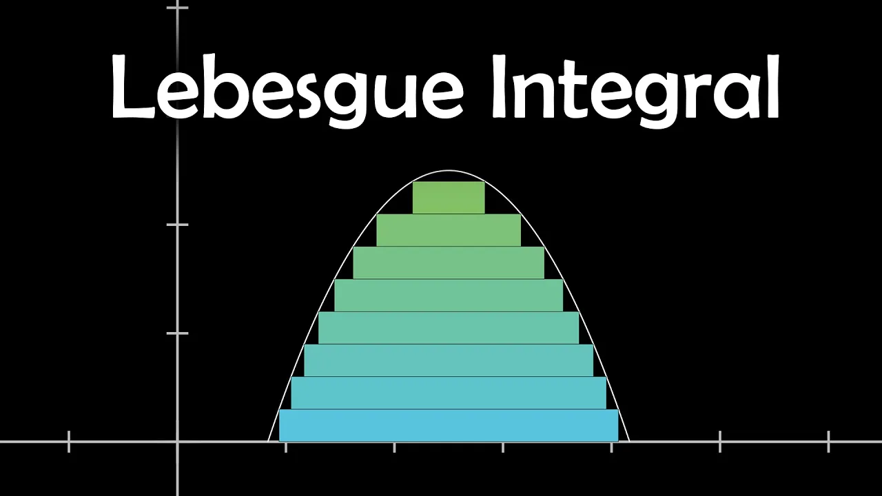
A horizontal integral?! Introduction to Lebesgue Integration
373.4K
Lebesgue integration, developed by French mathematician Henri Lebesgue, provides a more powerful alternative to Riemann integration by measuring the size of sets in the range (y-axis) rather than partitioning the domain (x-axis); this approach enables integration of highly discontinuous functions like the Dirichlet function (which equals 1 for irrationals and 0 for rationals) by summing the product of function values and the measure of their corresponding sets, and forms the foundation for modern probability theory and expected value calculations.
Click to watch →

En quoi l'Intégrale de LEBESGUE est-elle Supérieure à Celle de RIEMANN ? | Épisode 2
73.9K
The Riemann integral uses vertical partitions (intervals on the x-axis) and sums areas of rectangles taken sequentially while preserving the curve's order. The Lebesgue integral groups contributions by their heights (values), first counting all contributions at height y1, then y2, etc. This allows Lebesgue to handle complex bases including unions of intervals and countable sets like the rationals. The Lebesgue integral is less sensitive to discontinuities because it doesn't depend on the order of abscissas. Every properly Riemann-integrable function (continuous, piecewise continuous, regulated) is also Lebesgue-integrable with the same value, but Lebesgue extends to more functions.
Click to watch →
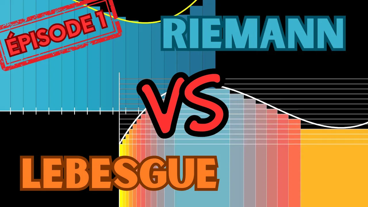
Qu'est-ce qu'une Aire Sous La Courbe ? | E01 - Introduction aux Intégrales de RIEMANN et de LEBESGUE
36.2K
Despite its strengths, the Riemann integral has significant limitations: it fails for highly discontinuous functions like the characteristic function of rationals, lacks powerful theorems for interchanging limits and integrals (requiring uniform convergence), and struggles with non-Euclidean spaces. The Lebesgue integral addresses these issues by subdividing the function's range (image) instead of its domain. Rather than approximating with horizontal rectangles, it groups curve portions by function values and approximates with vertical slices of constant height. This approach aggregates contributions of the same height together, creating a more robust integration framework that handles pathological functions and provides superior theoretical foundations.
Click to watch →

Lebesgue Integral Overview
109.8K
The Lebesgue integral is constructed by starting with indicator functions (which equal 1 on a set and 0 elsewhere), then defining integrals for simple functions as linear combinations of indicators, followed by approximating more general non-negative functions using limits of simple functions, and finally extending to all real-valued functions by decomposing them into positive and negative parts; this approach allows integration of a much broader class of functions than the Riemann integral, including those with discontinuities or unbounded behavior, and enables powerful convergence theorems like the Dominated Convergence Theorem.
Click to watch →

Understanding Measure Theory and the Lebesgue Integral
88.2K
The Lebesgue Integral extends integration beyond Riemann integration by partitioning the function's range rather than its domain, enabling integration of functions with severe discontinuities like the Dirichlet function; it is built on measure theory, which defines measurable sets through sigma algebras and assigns measures (generalizing length, area, volume) to them, allowing rigorous treatment of limits and convergence via theorems like the Monotone Convergence Theorem and Dominated Convergence Theorem, and forms the mathematical foundation for probability theory where measure spaces correspond to probability spaces.
Click to watch →
Course Intro
Integral Defs
Integrability
Partition Sums
Sum Components
Limit Forms
Riemann Sums
Result Derive
Final Limit
Course Intro
0:02- 1
Covers engineering math topics like algebra and complex analysis.
- 2
Starts explaining real-valued bounded functions on a closed interval.
Lebesgue Integration
While Riemann integration (relying on upper and lower Darboux sums) is foundational, it has major limitations in advanced mathematical analysis. It struggles with highly discontinuous functions—for example, the Dirichlet function (which is 1 on rationals and 0 on irrationals) is not Riemann integrable. Lebesgue integration overcomes this by partitioning the function's range rather than its domain, utilizing measure theory to define the integral. This alternative framework allows a much broader class of functions to be integrated. Additionally, Lebesgue integration provides powerful convergence theorems (like the Monotone and Dominated Convergence Theorems) that allow the interchange of limits and integrals under much weaker conditions than the strict uniform convergence required by Riemann integration, making it the standard in modern analysis and probability.
Understanding of bounded functions on closed and bounded intervals [a, b].
Concepts of Supremum (Least Upper Bound) and Infimum (Greatest Lower Bound) of a set of real numbers.
The definition of a partition of an interval, including subintervals and partition norm/mesh.
The construction and calculation of Upper and Lower Darboux Sums for a given partition.
The formal definition of Riemann Integrability (proving when the upper and lower Riemann integrals are equal).
Riemann's Criterion for integrability and its application to specific function classes.
The Fundamental Theorem of Calculus, bridging the gap between differentiation and Riemann integration.
The classification of integrable functions (e.g., continuous functions, monotonic functions, and functions with finitely many discontinuities).
Transitioning to Lebesgue Integration to handle highly discontinuous functions where Riemann integration fails.
412.1K views7.2Klikes18:49@gajendrapurohitOriginal Release: 2021-02-10
[Music] [Music] hello students videos uplo for engineering mathematics B albra complex analysis numeric analysis and linear algebra mathematics operation the L then partial differential equational equation and FX the real Val bounded function defined on a Clos interval AB FX real Val f the low integ the lower integral of FX or Clos interval AB is the supremum of this LF don't worry about that it will be good for you right P AB right and it is denoted by this to be FX DX supremum of lfp where P def right over AB is the infinum value of UF upper belongs to and it ised by a FX ax right this function is or lower right so a bounded function f is set to beable or Clos interval AB if upper limit upper is equal to lower inter right 1 + 2+ n upon n + 1 by 2 Su n s 1 sare 2 sare 3 sare n sare n into n + 1 2 n + 1 by 6 summ n 1 1 Cube 2 Cube 3 Cube Up 2 n n into n + 1 by 2 Al beta al+ 2 Bet f is defined on Clos inter then FX equal K FX k for all X belongs to AB where K is constant a exactly X1 the sub interal of this AB [Music] r XR XR right right r 1 right Mr XR minus XR right right into XR XR of the inter right1 x3 - x- x max X lowor FXX UF [Music] canc same to same concept d right Upp lius lower limit 1 1 by one 1 by n 1 by n 1 by add right Z 1 by 1 by n 2 byn 3 by R right right Sox X Mr upon R by or R R-1 upon n or R by n right Rus r- 1 upon + 1 2 XF n + 2 ler r r sorry n right 2 right n-1 upon into N - 2 upon 2 right limit n to infite nus 1 into N - 2 upon 2 n² N Li n to infity 1 1 2 2 0 to 1 FX FX DX andal 0 to 1 FXX l cility so thank you so much for watching me thank you
Up Next
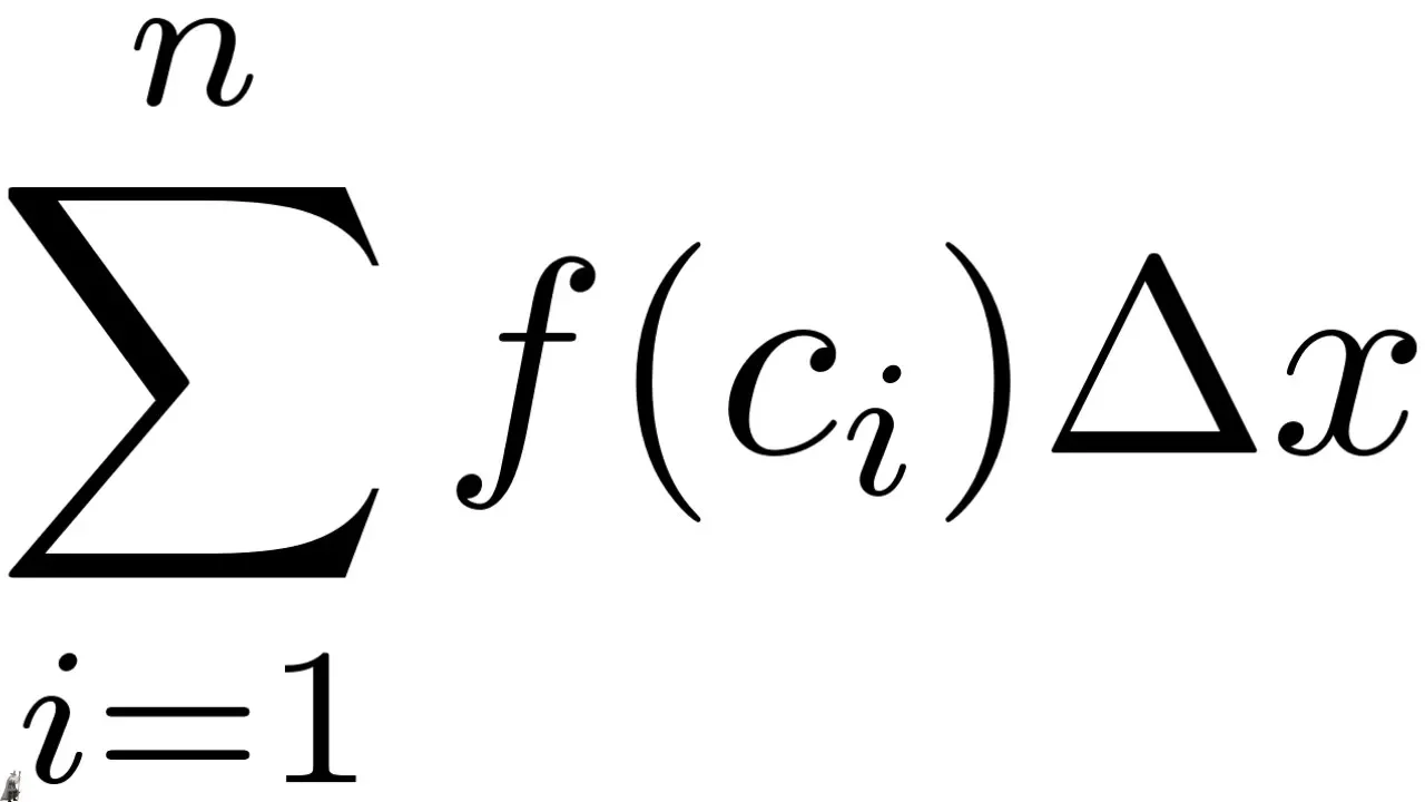
12:13
Riemann Integral Formal Construction and Definite Integrals
@TheMathSorcerer
2K views•2019-09-08

4:43
Elliptic Curve Cryptography Explained: ECC, ECDSA, ECDH
@PracticalNetworking
28.5K views•2024-10-21

10:44
Fourier Series Introduction: The Big Idea Explained
@DrTrefor
387K views•2021-05-03

6:00
The Mathematical Impossibility of Accurate World Maps
@Vox
23.3M views•2016-12-02
Related Study Plans & Knowledge Roadmaps
Structured learning paths in Mathematics
mathematics
Tensor Calculus: Vectors to Riemann Curvature
01Mathematical Foundations: Linear Algebra & Calculus
02Covectors, Dual Spaces, and Tensor Basics
03The Metric Tensor and Index Gymnastics
+ 2 more learning modules
40h5 modules
Explore Roadmap
mathematics
Gödel's Incompleteness: Logic, Proofs & Limits
01Introduction to Formal Systems & Hilbert's Dream
02Set Theory, Cardinality, and Cantor's Diagonal Argument
03Arithmetization and Gödel Numbering
+ 2 more learning modules
14h5 modules
Explore Roadmap
mathematics
Galois Theory: Fields, Groups & Solvability
01Foundations of Abstract Algebra: Groups & Fields
02Polynomials & Field Extensions
03Splitting Fields & Symmetries
+ 2 more learning modules
24h5 modules
Explore Roadmap
mathematics
Non-Euclidean Geometry: Models & Geodesics
01Euclid's Fifth Postulate and the Birth of New Geometries
02Hyperbolic Space and the Poincaré Disk Model
03Geodesics: Defining Straight Lines in Curved Spaces
+ 2 more learning modules
15h5 modules
Explore Roadmap