


![[s2 | 2025] Математический анализ, К. В. Правдин, лекция 25](https://i.ytimg.com/vi/kBUpNIgXNzY/maxresdefault.jpg)











![[s4 | 2026] Математический анализ, Трифанова Е. С., лекция 1](https://i.ytimg.com/vi/-E4ojpmOaLQ/maxresdefault.jpg)










The Lebesgue integral generalizes the Riemann integral by partitioning the codomain (y-axis) of a function and measuring the pre-image sets of these partitions, rather than partitioning the domain (x-axis); this approach eliminates the Riemann integral's limitations in higher dimensions, its strict continuity requirements, and its inability to interchange limits with integrals except under uniform convergence, making it more robust and flexible for modern mathematical applications.
Riemann vs Lebesgue Integral: Motivation and Key Differences
Added:Definition and formulation of the Riemann integral, including partitions, step functions, and upper/lower Darboux sums.
Fundamental concepts of real analysis, such as pointwise and uniform convergence of function sequences.
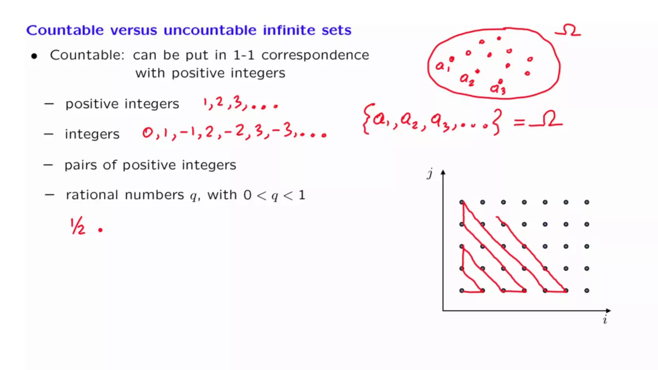
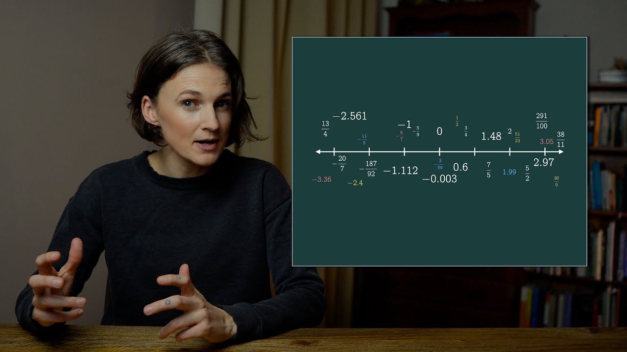
Basic set theory, specifically the distinction between countable and uncountable sets (e.g., the cardinality of rational vs. irrational numbers).
Intuitive understanding of 'measure' or length of intervals on the real number line.
Formal construction of Lebesgue measure, outer measure, and the sigma-algebra of Lebesgue measurable sets.
The core convergence theorems of Lebesgue integration, specifically the Monotone Convergence Theorem and the Dominated Convergence Theorem.
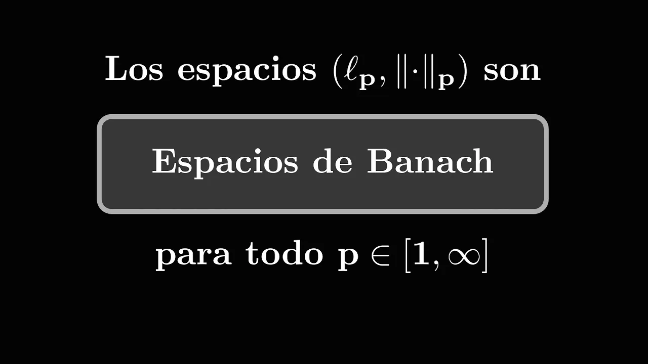
Introduction to L^p spaces, completeness (Banach spaces), and their role in functional analysis.
Abstract measure theory and integration on general measure spaces, including product measures and Fubini's Theorem.
14K views395likes19:39Original Release: 2022-12-12
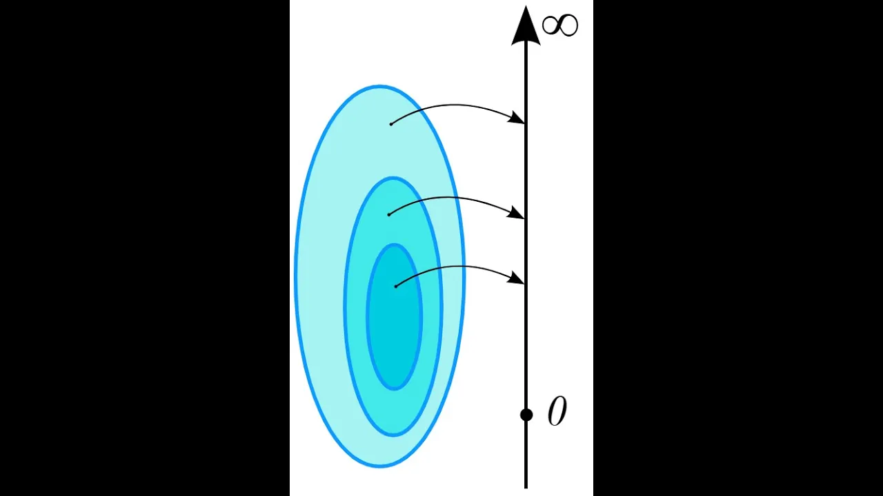
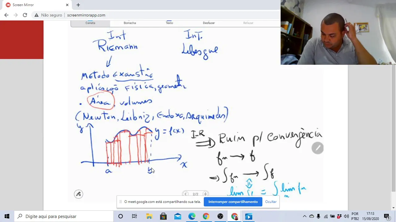
hello and welcome to Iman integral versus slipback integral often students ask me why we have two integral Notions at all or why we need the back intercool when we already have the Riemann integral in this video I explained why we go from the classical integral definition which is the Riemann integral to the more modern one which is still a back integral however let us first start with the women integral here we want to integrate a function f that starts from R and goes into r so a normal function defined on the realign and with values in the real line and as you should know this integral is related to the calculation of an area below a graph so let me do a rough drawing of this graph for the function f here and consider an interval on the V line so maybe we start with a and go to B then we are talking about this area below the graph so exactly this one in short this means the Riemann integral of the function f from the integral a b is related to this area here therefore we have the well-known idea to choose the partition of the x-axis and to approximate this area by choosing rectangles and this approximation is known as the lower sum or the upper sum so what I saw here is the well-known lower sum and if we now choose finer and finer petitions we call this limit of the lower upper sums the Riemann integral if the limit is well defined well this was a short summary of The Riemann integral and now we immediately find some problems here these problems give us a reason to Define another integral notion firstly it is difficult to expand the Riemann integral to higher dimensions yes you can expand it to higher Dimensions so it is possible but it's very laborious for example if we would have a 2 here this means that the x-axis here is now a two dimensional space so we can't use rectangles for the partition of course we now could use cuboids so if this is the two-dimensional space in the domain of definition this R2 then our partition is now just rectangles and this plane and our integral approximation now is given by cuboids so maybe in this way as you can see it gets very technical and it will be much more work with this addition to the dimension just one more Dimension but you have to do much more work for example to build the limit process in the end this is directly clear if we consider the domain of definition here in the one-dimensional case we only have an interval so this is an easy thing since it starts with a and ends with B just an interval but even if we add only one dimension more so here's the picture X1 X2 and F of X1 X2 so even if we just add one dimension there are a lot of more possibilities for example the domain of definition for the function could be a circle in this plane so let us focus on the domain of definition now so I throw another picture just the X1 and X2 axis and then we find the circle just there what we now want to do is choose a partition of the circle and put the cuboids above however of course this is not exactly possible so we can put rectangles inside the circle here but as you can see we even need a limit process to approximate a circle in domain of definition again I said it is feasible but it's a lot more technical work in summary this is one problem of the Riemann integral we directly understand it is much more work to do this in higher dimensions the second problem of the wema integral and what you should know from this one-dimensional case is that we need some continuity property for the functions we want to integrate in other words we have some dependence on continuity we call that in the best case the function we want to integrate should be continuous then we don't have any problems however if we have discontinuity points then there should be only finitely many of them but if we have infinitely many it can destroy the integrability of the function I hope you know the typical example so an easy function that you can't integrate using do we mon integral hence the dependency is indeed a disadvantage of the Riemann integral now the most important disadvantage of the Riemann integral is the relationship to limit processes the question is here in which situations is it allowed to Interchange some limit processes or in other words can I pull a limit sign inside the integral sign so let me tell this in an example so we have to limit n to infinity and we integrate a function from A to B so this is a sequence of functions FN and we integrate them with respect to X the question is then when is it allowed to pull will it push the limit inside the integral so when does this equality hold for the rieman integral we don't have many possibilities here we always need the uniform convergence of this sequence of function only then we know that it is allowed to pull the limit inside the integral however this uniform convergence is a very strong notion and in some sense related to the continuity again and therefore we want to weaken this notion indeed we have a lot of examples where there's no uniform convergence of the sequence of functions at all and we still have the same result on both sides hence we know it should be possible to generalize this convergence theorem however not by using the we monitor call to we monitor call is just not flexible enough to prove such an Convergence Theory well these are three important points that show the difficulties we may have when we use the remon integral most importantly we have a wish to the generalization to higher Dimensions so we want an integral notion that is not restricted to one dimension so we don't want to do all the work again if we just change the space of the domain of definition here we want an integral that works in every Dimension the same in order to understand this generalization we need more technical details hence I would suggest we start with the Riemann integral again we do some sketch so we have the X and the y-axis we also have a function where I draw the graph in green so we have a function with values in the real numbers for the women in the Chrome we now choose a partition of the x-axis as before and now we can calculate the upper and the lower sum here I have torn the lower sum which means that we take the infimum in each sub-interval for the height of the rectangles and for the upper sum we will take the supremum so here for example this rectangle hence we get the upper sum if the difference between the upper and the lower sum can be made arbitrally small for an finer partition then we can Define the Riemann integral then you can Define it as the supremum of the lower sums or the infimum of the upper sums this is then the same value and this value is called the Riemann integral for the function f in the interval a b in order to do this it was necessary that we have a function that goes from the real numbers inside the real numbers otherwise we can't do the partition of the x-axis and we don't have a height here the idea of the back integral is now different as you have seen before it was very restrictive to find a petition of the domain of definition if it is not R itself so if we for example have a three-dimensional space then we can't find a partition easily but we met still in the real numbers so the right hand side is still the same since we consider functions so functions with values and the real numbers so this is the same the left hand side is not the same this means that the domain of definition the left hand side here can be very high dimensional or even very abstract and therefore we don't know what a meaningful partition of the left hand side should be just because we don't have these simple intervals in a high dimensional or abstract space however on the right hand side we still find the real numbers the one-dimensional space of the real numbers so instead of find the partition of the x-axis it would be easier to justify the petition of the y-axis and indeed this is what the back integral does although this is not the way the back in the coil is normally introduced however it is still a very good idea to visualize the back integral so let us throw the graph again and keep in mind the x-axis may be high dimensional or even abstract but the y-axis is still the real line and that is what we decompose now since this is only the real line we can find the same interval partition as before so we choose some values and Define some intervals here so this is a partition of the realign as we did before in the real integral on the x-axis so maybe we call these partition elements CI where we in the real integral we usually denote them by x i maybe as in my mind of what we did in the rim and equal was we defined an upper sum of some partition of the x-axis so you would write U of the partition and this is the sum of all the rectangles which means the sum and then you choose the supremum inside the interval times the length of this interval so times the length of your partition so maybe Delta x i and you can do the same for the lower sum then again be sum all the rectangles up but each one is given by the infimum inside the given interval infimum infimum of f of x times the length of the rectangle so times the length of the interval there so I call it Delta x i and this way we usually Define the V1 integral however now we want to decompose the y-axis for getting the back integral now we get the following picture for example this line here so this value gives you this line here and this line here now we want to find all the parts of the function that lie between these two lines so meaning inside this interval or in the real line this means that we don't draw rectangles as before but we look which part of the functions lie inside these two lines then we find here that we have one part on the left hand side so we find all the arguments in X that lie in this set I'll send two values inside this interval by the function f and we also have here a part of the function so we can project it again down to the x-axis and then we find okay all the arguments in X here are getting sent to the interval now these two parts are associated to the decomposition the partition of the y-axis CI we shows this is similar to the idea of the Riemann integral but we immediately see that the decomposition of t x axis below here is not connected so we have different sets that are not connected in intervals as before and this is the whole idea instead of choosing a fixed partition of the x-axis we now choose a partition of the y-axis of the values of the function and then we get a useful partition of the x-axis that we can work with now the next question could be how to measure these lengths on the x-axis below therefore on the domain of definition which is here uh free but it could be some space we need a so-called measure we want to measure volumes in this space this means that we want to measure the size of sets inside this space so for example if the space is R we measure lengths in R2 we would measure areas in R3 it would be indeed we measure volumes of sets uh but in abstract sense we always speak of volumes hence on the x-axis here we could choose a general measure space we just have to know how to measure the size of sets or the volume of sets and such a measure space is usually denoted by Omega this means in the end we will have an integral that works on all functions that are defined on some measure space Omega indeed this is all we need to define the integral now you see how we could Define an upper sum in some sense so we take the c i Here and Now I want to see I to be this one so maybe I do a little picture so the CI is this swipe here so this would be an upper sum for the integral if we know the measure of the two sets together of course these blue sets are just the pre-image of this interval under the function f so maybe we'll just call it a now if I call the measure we have here in our measure space just by mu then we can calculate this generalized rectangle it is c i so the height times the length on the bottom this is the measure of our set hey now we have one part of the whole integral and now we can do this for the whole partition so we have a finite sum over I of course I should put an index I for a for the pre-image as well and then we have a sum and since we chose a finer partition of the y-axis we have a finite sum here and it is the upper sum or the lower sum depending which CI we shows here then again with some limit process with finer partitions we will get double back integral and usually denoted by F the moon since now it's depending on the measure we chose on the x-axis indeed this construction now works for arbitrary measure spaces since the x-axis doesn't need a petition anymore we just need a partition of the axis that is R anyway however in this case we really need the notion of measure even in one dimension so here we know what the length of the sub interval is it's just the difference between the right hand side and the left hand side but here we need more or in other words in the reamer integral we just measure lengths of intervals but in the back integral we can have any fragmentation and we have to know the measure of this fragmentation but if we know how to measure any set in the real line then we have a very robust integral definition well this generalizes the Riemann integral and eliminates all problems we had in higher Dimensions since this mineral Theory Works in every Dimension as you want you just have to know how to measure volumes and also the dependence of the continuity is gone since now we can measure the size of the set of the points of discontinuity for example if we have infinitely many points of discontinuity but the measure of all these points so the measure of the set of all the points is zero we don't have a problem and the definition of the integral at all and also for the last point so these limit processes we have good answers for we will see that we have very good limit theorems that describe these limit processes for the back integral even strong results for the one dimensional case but also in the general case of measure spaces okay to sum it up the Riemann integral is the classical notion it may be easier to understand at the beginning level but in the end everyone wants to work with the the back integral thank you very much and see you next time [Music]
Up Next
11:48
Borel Sigma Algebras Explained | Measure Theory 2
@brightsideofmaths
284.2K views•2019-07-16

4:43
Elliptic Curve Cryptography Explained: ECC, ECDSA, ECDH
@PracticalNetworking
28.5K views•2024-10-21
8:22
Laurent Series Explained | Complex Analysis
@brightsideofmaths
52.4K views•2022-04-06

6:00
The Mathematical Impossibility of Accurate World Maps
@Vox
23.3M views•2016-12-02
Related Study Plans & Knowledge Roadmaps
Structured learning paths in Mathematics
mathematics
Tensor Calculus: Vectors to Riemann Curvature
01Mathematical Foundations: Linear Algebra & Calculus
02Covectors, Dual Spaces, and Tensor Basics
03The Metric Tensor and Index Gymnastics
+ 2 more learning modules
40h5 modules
Explore Roadmap
mathematics
Gödel's Incompleteness: Logic, Proofs & Limits
01Introduction to Formal Systems & Hilbert's Dream
02Set Theory, Cardinality, and Cantor's Diagonal Argument
03Arithmetization and Gödel Numbering
+ 2 more learning modules
14h5 modules
Explore Roadmap
mathematics
Galois Theory: Fields, Groups & Solvability
01Foundations of Abstract Algebra: Groups & Fields
02Polynomials & Field Extensions
03Splitting Fields & Symmetries
+ 2 more learning modules
24h5 modules
Explore Roadmap
mathematics
Non-Euclidean Geometry: Models & Geodesics
01Euclid's Fifth Postulate and the Birth of New Geometries
02Hyperbolic Space and the Poincaré Disk Model
03Geodesics: Defining Straight Lines in Curved Spaces
+ 2 more learning modules
15h5 modules
Explore Roadmap