This video demonstrates how to set up and control an aerofoil in a wind tunnel using a two-force component system, including placing the airfoil on standard connections, connecting data cables to associated ports, installing lift and drag load cells, and controlling the angle of attack by adjusting the airflow direction.
How to Set Up and Control Aerofoil Shapes in a Wind Tunnel
Added:Deep Dive
Fundamental aerodynamics concepts including lift, drag, and the relationship between velocity and pressure (Bernoulli's principle).

BHPA Pilot rating - Theory of Flight
13.4K
Lift is generated through Bernoulli's principle: accelerating airflow over a curved surface reduces pressure. An airfoil deforms airflow by accelerating it at the top surface and slowing it at the bottom, creating pressure differential. Approximately 2/3 of lift depression occurs at the top surface. The center of pressure is the theoretical point where all pressure forces converge. Angle of attack—the angle between chord line and airflow—is critical: stall occurs when angle of attack becomes too high, causing airflow separation. Lift and drag are perpendicular forces; creating lift always creates drag. Induced drag comes from pressure differences at wingtips, while parasitic drag (friction and form drag) increases with the square of speed. Total drag is minimized when induced equals parasitic drag.
Click to watch →
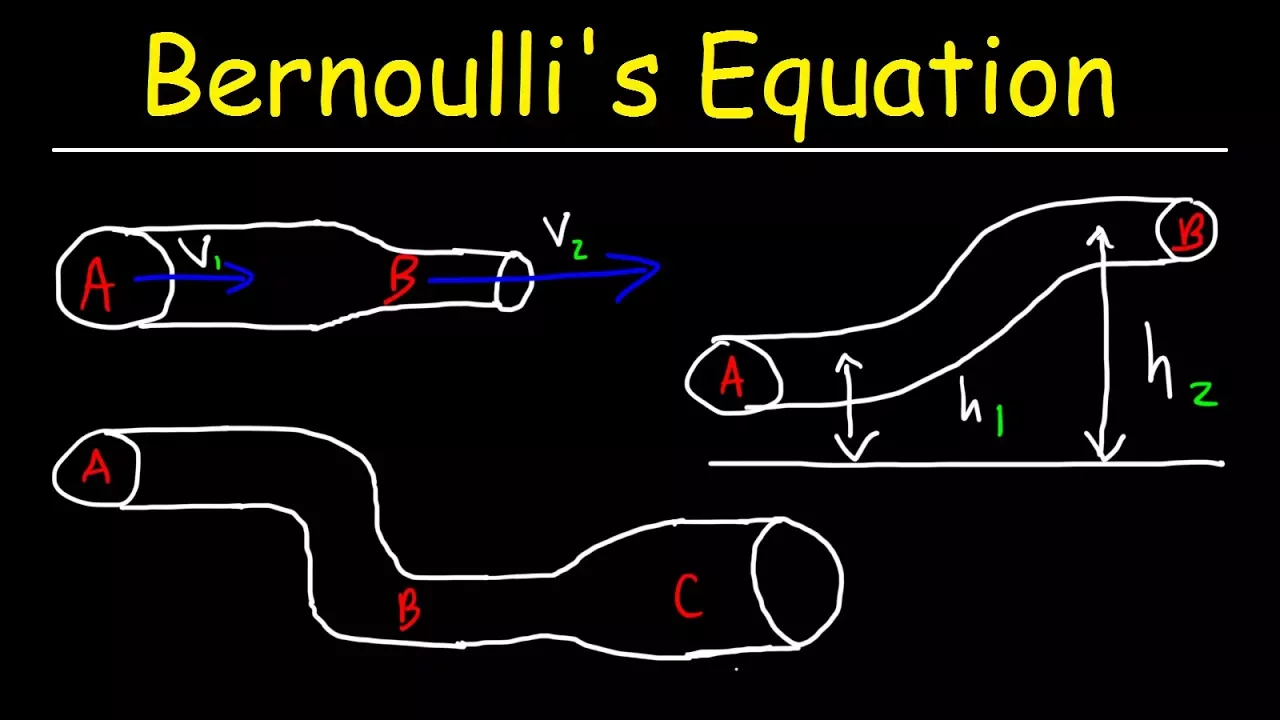
Bernoulli's Equation Example Problems, Fluid Mechanics - Physics
808.9K
Bernoulli's principle describes the relationship between fluid speed, pressure, and elevation. Key concepts include: (1) Continuity equation (A₁v₁ = A₂v₂) shows that decreasing pipe area increases fluid velocity; (2) Inverse relationship between pressure and velocity—faster-moving fluid has lower pressure; (3) Pressure decreases when fluid accelerates due to net force from pressure differences; (4) For horizontal pipes, pressure drop occurs as velocity increases. These principles explain why airplane wings generate lift and how venturi meters measure flow rates.
Click to watch →

Теория и тактика парящих полётов. Лекция 1
5.9K
Bernoulli's principle states that in steady flow of an incompressible fluid, an increase in velocity occurs simultaneously with a decrease in pressure. Static pressure is the pressure exerted by a fluid at rest, while dynamic pressure is associated with fluid motion (½ρv²). The total pressure is the sum of static and dynamic pressure. This inverse relationship between velocity and pressure is the fundamental mechanism behind lift generation on airfoils.
Click to watch →

Fluida Dinamis Part 4 Penerapan asas bernoulli 2 gaya angkat pesawat
41.1K
Aircraft generate lift through pressure differences created by air flow over wings. The lift force equals the pressure difference between bottom and top surfaces multiplied by wing area. Bernoulli's principle explains this: for thin wings with negligible height difference, pressure plus kinetic energy remains constant. This means higher velocity above the wing creates lower pressure, generating upward lift. The key relationship is that velocity above the wing must exceed velocity below for lift to occur.
Click to watch →
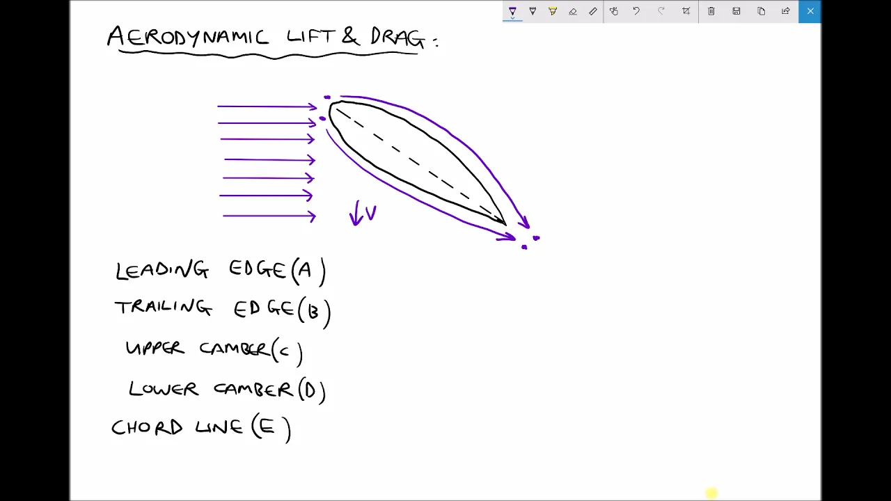
Effects of Aerodymanic Lift & Drag Forces on an Aerofoil
5.9K
According to Bernoulli's principle, air traveling across the lower camber has a shorter distance to travel in the same time, resulting in lower velocity. Conversely, air traveling over the upper camber has a greater distance to travel, resulting in higher velocity. When air slows down, pressure increases to compensate while maintaining total energy conservation. When air speeds up, pressure decreases. This creates a pressure differential where pressure is higher below the aerofoil and lower above it.
Click to watch →
Deep Dive
Basic anatomy of an aerofoil, such as chord line, camber, angle of attack, leading edge, and trailing edge.
Theory of flight
644
An aerofoil has key anatomical features: leading edge, trailing edge, camber, and chord line. The chord line runs from the furthest point of the leading edge to the aft point of the trailing edge, and is essential because angle of attack is measured between relative airflow and the chord line. Angle of attack is the fundamental factor determining whether an aircraft flies or stalls. Regardless of aircraft type, it will have an aerofoil, chord line, and relative airflow, making angle of attack universally important. The critical angle of attack is where airflow can no longer cling to the wing surface, causing a stall. Understanding these concepts is essential for all pilots.
Click to watch →
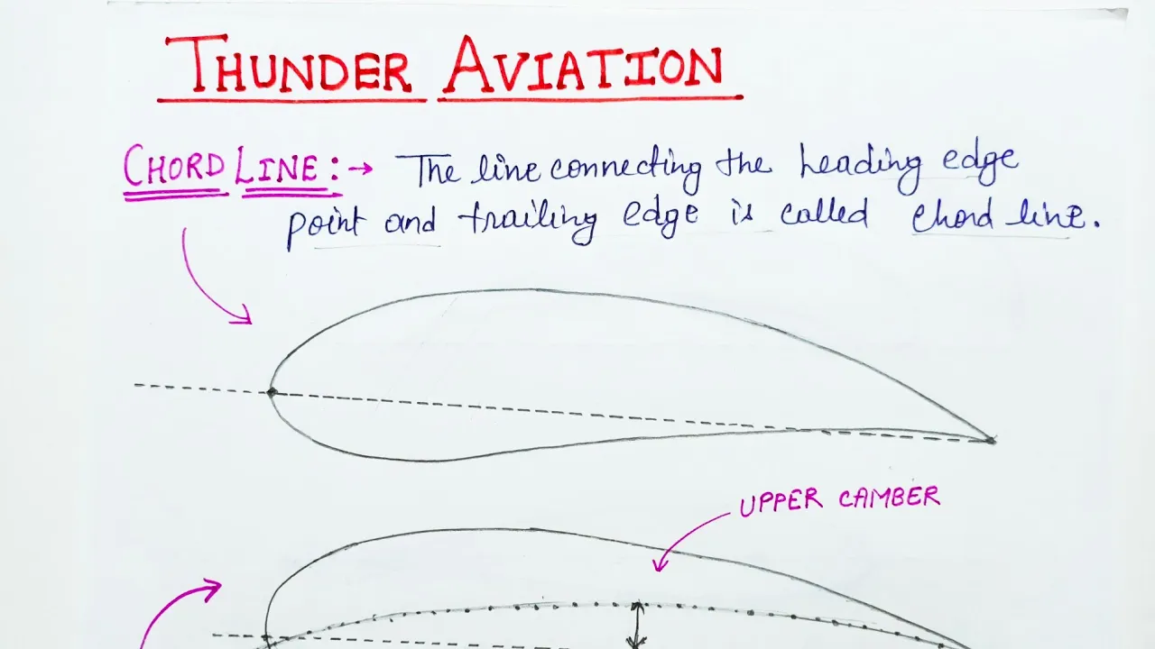
Chord Line | Camber | Angle Of Attack | Basic Aerodynamics| #aviation #aircraft #ame
3.3K
In basic aerodynamics, the chord line connects the leading edge and trailing edge of an airfoil, the mean camber line is equidistant from both upper and lower surfaces, camber is the distance between the mean camber line and chord line, and the angle of attack is the angle between the chord line and the relative wind direction.
Click to watch →

Understanding Aerodynamic Lift
1.9M
Airfoil profiles are defined by several key parameters. The forward-most edge is called the leading edge, while the trailing edge is at the back. A straight line connecting these points forms the chord line. The angle between the chord line and the flow direction is the angle of attack. The mean camber line is drawn midway between the upper and lower surfaces. Camber describes how curved an airfoil is, with positive camber indicating upward curvature, negative camber indicating downward curvature, and zero camber for symmetrical airfoils. Both camber and angle of attack significantly influence lift generation.
Click to watch →

Airplane Aerodynamics Lecture | Private Pilot Ground School
3.6M
Key airfoil terms include: leading edge (front of wing), trailing edge (back of wing), chord line (straight line from leading to trailing edge), and camber (curvature of the airfoil). The chord line serves as a reference for measuring angle of attack. Camber describes how curved the upper and lower surfaces are, with greater curvature typically increasing lift-generating capability.
Click to watch →

Types of Aerofoils and uses
133
The chord line connects the leading and trailing edges of an airfoil. The camber line is the curve equidistant from the upper and lower surfaces. The angle of attack is the angle between the chord line and relative airflow. Positive camber (curved upper surface) generates lift at zero angle of attack. Negative camber (curved lower surface) is rarely used. Symmetric airfoils have identical upper and lower surfaces.
Click to watch →
Deep Dive
General wind tunnel operation principles, including flow conditioning, test section velocity, and boundary layer formation.
![[Aeronáutica General] Clase virtual N° 7](https://i.ytimg.com/vi/UhI9umxx4Ec/maxresdefault.jpg)
[Aeronáutica General] Clase virtual N° 7
178
A wind tunnel consists of key components: inlet lip, settling chamber, convergent, propeller group, and test section. The settling chamber maintains constant velocity, while the convergent accelerates flow. Two fundamental equations govern tunnel analysis: the continuity equation (area × velocity = constant) and Bernoulli's equation (total pressure constant along streamlines). In an open test section, static pressure equals atmospheric pressure. The honeycomb structure aligns velocity vectors with the tunnel axis. Wire meshes straighten flow and produce pressure losses proportional to velocity squared. The convergent must avoid abrupt changes to prevent flow separation. The test section has maximum velocity and minimum static pressure. Blockage limits are 10% for open and 5% for closed test sections. Wind tunnels are classified by: (1) Impulsion vs. Aspiration (propeller upstream or downstream), (2) Open vs. Closed test section, (3) Circuit open vs. circuit closed. The boundary layer is the region where viscous effects are significant, requiring a fluid flow and solid surface. The no-slip condition applies: velocity is zero at the wall. As distance from the wall increases, velocity increases until reaching free stream velocity. The boundary layer thickness (δ) is defined where velocity reaches 99% of free stream velocity. At the leading edge, thickness is zero. Initially, flow is laminar (ordered). At a critical Reynolds number, transition to turbulent flow occurs. Turbulent boundary layers grow faster and offer more friction resistance.
Click to watch →

How Wind Tunnels Work: Components & Design
54.3K
Wind tunnels are aerodynamic testing facilities that force air across objects to study their aerodynamic properties; they consist of several key components including a fan to push air, turning vanes to straighten flow, a settling chamber with honeycomb structures and screens to reduce turbulence and swirl, a contraction to increase flow velocity before the test section, and a diffuser to slow the air down again, with the goal of achieving low turbulence intensity, uniform flow velocity, and thin boundary layer at the test section.
Click to watch →
Research Opportunities in the NHERI Boundary Layer Wind Tunnel-Jennifer Bridge-10-19-23
213
Boundary layer wind tunnels simulate atmospheric boundary layer conditions for structural testing. The facility uses eight axial fans to drive airflow through honeycomb straighteners, optional Irwin spires for large-scale mixing, and roughness elements in the development section to grow the boundary layer. Standard tests include flow characterization (velocity probes), rigid pressure-tapped models, rigid models with high-frequency force balances measuring reaction forces, aeroelastic models accounting for structural flexibility, and cyberphysical models where characteristics change in real-time. Limitations include Reynolds number mismatch, inability to simulate large-scale turbulence effectively, usable profiles only up to ~25% of gradient height, and challenges with stationary/non-neutral profiles and higher-order flow characteristics.
Click to watch →
![[Aeronáutica General] Clase Virtual N°13](https://i.ytimg.com/vi/afU7aVIrCyY/maxresdefault.jpg)
[Aeronáutica General] Clase Virtual N°13
145
This segment introduces the wind tunnel practical exercise. The instructor explains the main components: (1) Diffuser (grupo propulsor) at the bottom providing airflow; (2) Test section (cámara de ensayo) for experiments; (3) Settling chamber (cámara de tranquilización) ensuring uniform flow; (4) Convergent accelerating airflow; (5) Diffuser decelerating airflow after the test section. The instructor describes operating conditions: subsonic, continuous operation, open circuit with aspiration. The settling chamber has the largest diameter (lowest velocity), while the test section has the smallest diameter (highest velocity). The airflow direction is from left to right, and the test section is closed with an aluminum wall.
Click to watch →

How Does A NASCAR Wind Tunnel ACTUALLY Work? Behind The Scenes in an Official Testing Facility!
42.5K
A wind tunnel is a machine that blows air on an object and accurately measures the effects. Design depends on the test object: airplanes need large tunnels with high speeds, while smaller objects like golf balls can use smaller tunnels. The test section must balance size - small enough for high speeds but large enough to avoid restricting airflow. The contraction section (4:1 ratio) accelerates air to 130 mph, while the diffuser recovers energy efficiently. Fans are placed at the rear to ensure smooth, uniform airflow rather than turbulent air from the front. The honeycomb section straightens air as it turns corners, functioning like an aerodynamic lens. Every air particle is a vector requiring correct angle and speed. Reynolds number determines when airflow qualities become consistent - for full-sized cars, speeds above 100 mph produce consistent air flow qualities. Wind tunnel design uses spreadsheets (Excel) as calculation tools, generating 3D point clouds that define the tunnel shape. Wind tunnels are bolted to the earth and don't need high-tech materials like carbon fiber or titanium. Construction uses concrete floors, steel I-beams, and wooden spars - similar to house building. Aerodynamics expertise comes from combining formal education with hands-on experience. Wind tunnels are designed for specific applications: the GM tunnel was for production cars, the NRC tunnel was all-purpose, neither was designed for race cars. Race car wind tunnels have unique requirements like very close ground clearance and dependence on airflow under the car. Boundary layer control keeps air moving along the floor because air naturally wants to slow down and stall. The system uses an air-to-air intercooler to keep injected air within 2° of ambient temperature. The HVAC system has 250 tons of cooling capacity. Wind tunnels generate significant heat because all electrical energy eventually turns into heat. Cars enter through a large door in the diffuser side. Curved walls reduce blockage effects by matching natural airflow around a car on a racetrack - air expands around the car and then collapses around it, creating a teardrop shape. Slotted walls serve as backup if the curved wall design doesn't work. The curved wall design was validated empirically by covering slots with aluminum covers. The tunnel uses 22 fans (18 in a rectangle plus 4 on top), each about 100 horsepower, selected for quiet operation near residential areas. Test cars are bolted to a balance in the basement, not supported by tires. The six-axis balance measures three forces (drag, side force, lift) and three moments (roll, yaw, pitch). Rolling roads move the floor at the same speed as airflow to simulate vehicle motion. Boundary layer is dead air along a stationary surface that drags down and stalls, creating a ramp of dead air that gets thicker downstream. Wind tunnels use suction (removing dead air) and blowing (energizing the boundary layer) to maintain thin boundary layers. Combining suction and blowing adds energy without changing mass flow, which is more efficient than moving floors. The entire floor system provides the correct boundary layer (zero thickness) regardless of how low the car sits. The front layer is a massive vacuum cleaner sucking away dead air. Multiple suction slots (1-5) incrementally remove air to keep the boundary layer thin. Forward-facing suction slots remove air while rearward-facing jets replace it. Tangential jets blow air out of very thin openings, speeding up air along the floor. The Kanda effect enables air to turn 90 degrees without raising surfaces above the flush floor. Tire rollers with electric motors spin at airflow speed, and turntables yaw the car about the front axle center line to simulate cornering conditions.
Click to watch →
Deep Dive
Introduction to measurement instruments commonly used in aerodynamic testing, such as manometers and force balances.

Manometers| pressure measuring instruments
358
Manometers are pressure measuring instruments that use liquid columns to measure pressure differences; a piezometer measures pressure at a single point, a U-tube manometer measures pressure difference between two points, and a differential manometer measures pressure difference between two points in a system.
Click to watch →

Calibration and Measurements in Wind tunnel
2.2K
Pressure measurement employs multiple technologies: manometers use liquid columns (mercury preferred for accuracy), barometers measure atmospheric pressure with one sealed end, and pressure transducers convert pressure to electrical signals for rapid, precise measurements. Wind tunnel balances measure aerodynamic forces with three main types: three-component balances measure forces along three axes, six-component balances measure at six discrete points (A-F) for comprehensive force distribution analysis, and external balances measure forces outside the primary test section. These integrated measurement systems enable comprehensive aerodynamic characterization in wind tunnel experiments.
Click to watch →
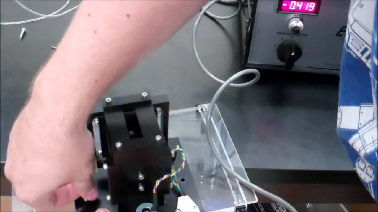
Measurements - Using the Airfoil with the Force Balance and the Wind Tunnel
12.3K
This video demonstrates how to calibrate and operate a lift and drag force balance system in a wind tunnel for aerodynamic measurements. The process involves setting up the force balance by mounting it upside down on a calibration fixture, connecting it to a digital readout, and applying known weights to calibrate the voltage output for both lift (up to 3.5 kg) and drag (up to 2.2 kg). After calibration, airfoils are mounted on the stinger using bolts and set screws, aligned to specific angles of attack, and tested in the wind tunnel. The voltage readings from the force balance are then converted to actual force values using the calibration curves established during the initial setup.
Click to watch →

Mass & Weight | Gravitational Field & Friction | Class 9 Physics Chapter 3 New Book| PCTB |
123
This section covers instruments for measuring mass and force. Mechanical balances compare mass by balancing objects with standard weights using a horizontal beam with knife edges. Types include mechanical balance and platform balance for heavy items. Electronic balances measure mass digitally without standard weights, displaying readings and calculating prices. Force meters (Newton meters) measure force directly in Newtons using a spring mechanism. The section explains working principles, reading methods, and differences between instruments.
Click to watch →

Азы аэродинамики переданные американцами Aerodynamic
8.6K
When an airplane flies steadily at constant velocity, forces are in equilibrium: drag equals thrust, and lift equals total weight. This allows determination of aircraft weight capacity and thrust requirements. To measure airfoil efficiency, small copper tubes are built into the model and connected to manometers. The manometer principle involves liquid in a reservoir that remains at constant level when pressure is constant. When pressure increases, liquid is forced into the reservoir, lowering the field level; when pressure decreases, liquid rises above the reservoir level. Each manometer can be connected to different points on the airfoil to record pressures at various locations.
Click to watch →
Prerequisite Knowledge
- Concept 01Fundamental aerodynamics concepts including lift, drag, and the relationship between velocity and pressure (Bernoulli's principle).
- Concept 02Basic anatomy of an aerofoil, such as chord line, camber, angle of attack, leading edge, and trailing edge.
- Concept 03General wind tunnel operation principles, including flow conditioning, test section velocity, and boundary layer formation.
- Concept 04Introduction to measurement instruments commonly used in aerodynamic testing, such as manometers and force balances.
Subsequent Learning
- Step 01Calculating and analyzing lift and drag coefficients (Cl and Cd) from raw experimental data.
- Step 02Utilizing flow visualization techniques (such as smoke wires, tufts, or dye injection) to identify boundary layer separation and aerodynamic stall.
- Step 03Comparing experimental wind tunnel results with Computational Fluid Dynamics (CFD) simulation data for validation.
- Step 04Investigating the effects of high-lift devices (like flaps and slats) and 3D wing phenomena (such as wingtip vortices and induced drag).
Setup Components
Connect Cables
Install Sensors
Ready Control
Set Angle
Setup Components
0:18Playing Section
- 1
Prepare force components and air foil for testing.
- 2
Mount air foil onto standard connections securely.
- 3
Tighten and lock equipment into place.
Computational Fluid Dynamics (CFD) as an Alternative to Physical Wind Tunnel Testing
While physical wind tunnel testing using apparatuses like the Matrix wind tunnel provides valuable empirical data, it is increasingly challenged and complemented by Computational Fluid Dynamics (CFD). Critics of exclusive physical testing point out that wind tunnels suffer from inherent limitations, such as wall interference, support-structure interference, and difficulties in achieving true flight-scale Reynolds numbers. In contrast, CFD offers virtual aerodynamic testing that eliminates these physical constraints. It allows researchers to rapidly iterate aerofoil designs, simulate extreme environmental conditions safely, and visualize flow fields in high resolution across the entire computational domain at a fraction of the operating cost of a physical tunnel. Consequently, modern aerodynamics often prioritizes computational simulation, utilizing wind tunnels primarily for final validation rather than primary design iteration.
Deep Dive
Calculating and analyzing lift and drag coefficients (Cl and Cd) from raw experimental data.

윙렛실험01
131
Lift and drag coefficients are calculated using the formulas: Cl = L / (0.5 * ρ * V² * S) and Cd = D / (0.5 * ρ * V² * S), where L is lift force, D is drag force, ρ is air density, V is velocity, and S is wing reference area. These dimensionless coefficients enable comparison of aerodynamic performance across different aircraft sizes and flight conditions. The experiment demonstrates how measured forces are converted into coefficients for meaningful aerodynamic analysis. Data processing involves coordinate transformations, force calculations, and coefficient determination using tools like Excel.
Click to watch →
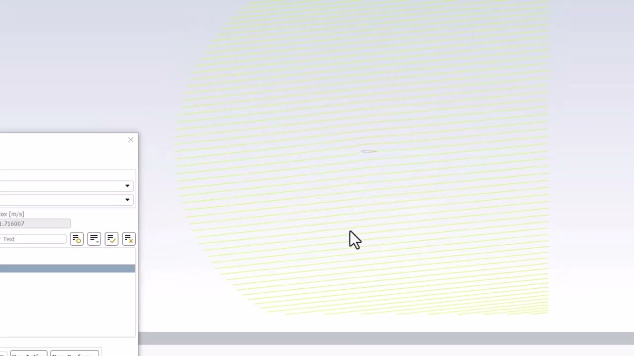
Numerical Results: Streamlines and Coefficients | Flow Over an Airfoil
1.5K
Lift and drag coefficients quantify aerodynamic forces on an airfoil. Expand Report Definitions in the tree structure and double-click CL (lift coefficient) to access its definition. Click compute to display the converged value in the console. Similarly, double-click CD (drag coefficient) and click compute. For this case, the converged lift coefficient is approximately 0.682, which compares reasonably with hand calculations and experimental data. The drag coefficient converges to about 0.06, very close to the expected value of zero, with small errors contributing to the difference. Mesh refinement would further improve these values by reducing numerical errors. These coefficients provide quantitative validation of the simulation results against theoretical expectations.
Click to watch →

Supermodified Racecar Wing design
9.8K
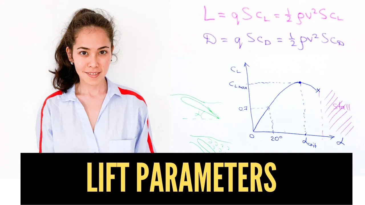
Lift coefficient (CL) is calculated as CL = Lift / (1/2 × ρ × v² × A), where ρ is air density, v is velocity, and A is wing area. Lift force = 1/2 × ρ × v² × A × CL. Using an online calculator with air density 1.225 kg/m³, velocity 100 mph, and 24 sq ft wing area, CL of 2.7 produces 1,656 pounds of lift. Increasing CL from 2.7 to 2.75 adds 30 pounds of lift. The same calculator computes drag from drag coefficient. Computer programs calculate theoretical performance in ideal conditions.
Click to watch →
Flow Past a Cylinder COMSOL Tutorial
11.3K
This segment derives and implements formulas for calculating drag and lift coefficients from simulation results. The lift coefficient (Cl) is calculated as: Cl = -2 × (reaction force in y-direction) / (ρ × U_mean² × A), where ρ is fluid density, U_mean is mean inflow velocity, and A is projected area. The drag coefficient (Cd) uses the x-component: Cd = -2 × (reaction force in x-direction) / (ρ × U_mean² × A). Both coefficients depend only on Reynolds number and object shape, not absolute size. The tutorial demonstrates implementing these expressions in COMSOL's point graph functionality, showing how simulation data is transformed into dimensionless coefficients for engineering analysis and comparison.
Click to watch →

AERO Coefficients of DRAG & LIFT equations & GUESS
122
The coefficient of lift (Cl) and coefficient of drag (Cd) are dimensionless ratios calculated using the formulas Cl = 2L/(A×ρ×V²) and Cd = 2D/(A×ρ×V²), where L is lift force, D is drag force, A is wing area, ρ is air density, and V is velocity; to solve for velocity, rearrange the formula and take the square root of the result.
Click to watch →
Deep Dive
Utilizing flow visualization techniques (such as smoke wires, tufts, or dye injection) to identify boundary layer separation and aerodynamic stall.
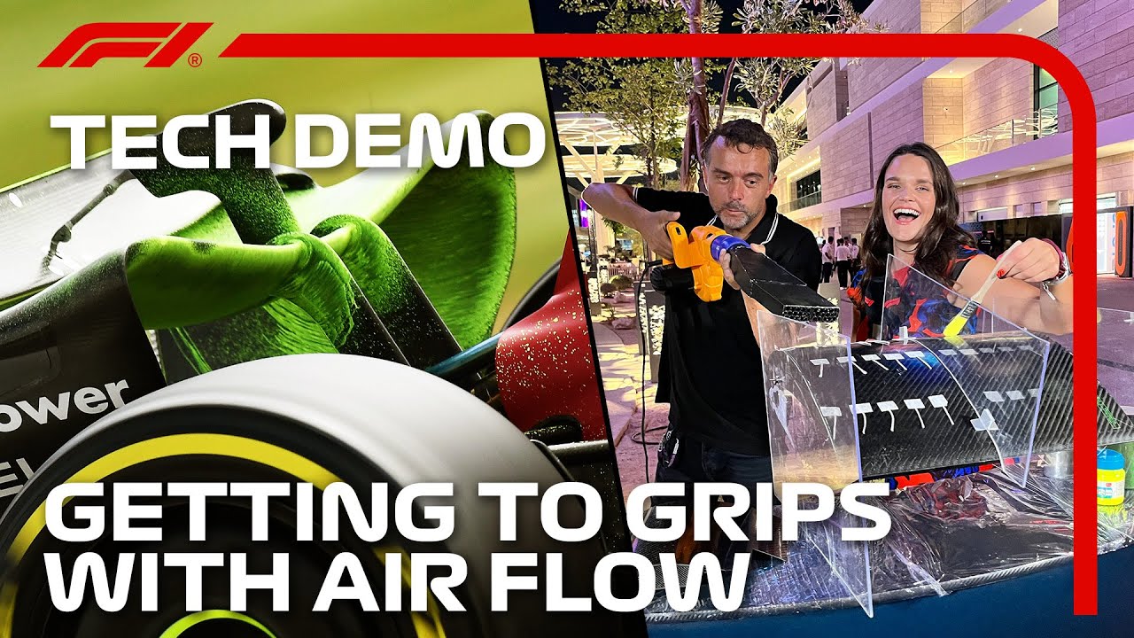
Going With The Flow: Understanding F1 Aerodynamics | Tech Talk | Crypto.com
131.6K
Teams use flow visualization to make invisible airflow visible. Strips attached to surfaces remain flat when air is attached but become chaotic when separation occurs. This reveals boundary layer behavior and flow separation, critical for understanding when surfaces stall. Teams test at different speeds and angles, including corners and braking zones, to observe how aerodynamics perform across racing conditions. Flow visualization uses colored powder mixed with light oil (flis), painted on car surfaces. When the oil evaporates on track, the powder reveals flow structures. Teams compare these visualizations with CFD simulations to verify aerodynamic performance and identify design issues.
Click to watch →

Wind tunnel pressure data for a NACA 0012 symmetric airfoil
54K
This section explores methods for visualizing and analyzing aerodynamic flow phenomena. Helium bubble visualization replaces smoke in closed-loop tunnels, revealing flow attachment and separation patterns. Tufts glued to airfoil surfaces provide qualitative flow indicators—laying flat when flow attaches, lifting when separation begins. Dynamic stall occurs when increasing angle of attack causes boundary layer detachment, forming a recirculation wake behind the airfoil. Visualization demonstrates how separation degrades lift and increases drag, with ensemble averaging of bubble images revealing detailed flow structures and their evolution with changing angles of attack.
Click to watch →

Boundary layer separation and stall
212K
As the angle of attack of an airfoil increases, the boundary layer flow initially stops and reverses direction (boundary layer separation), with the separation point moving forward along the airfoil; when this disturbance sufficiently disrupts the airflow, further increases in angle of attack produce decreasing rather than increasing lift, causing the wing to stall.
Click to watch →
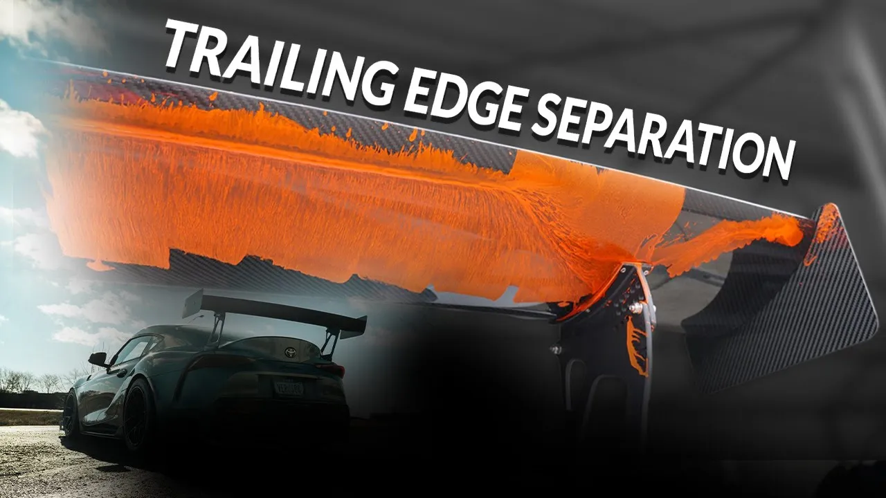
The issue with Flow Vis | Explained by Motorsports Engineers
3.1K
Flow visualization uses oil-based mixtures with fluorescent powder to reveal airflow patterns on surfaces. Wings experience two stall types: trailing edge stall (safe, gradual separation from rear moving forward) and leading edge stall (dangerous, rapid downforce loss). Separation follows tangential paths relative to the surface. Trailing edge stall is preferred for automotive wings because partial separation maintains significant downforce while providing warning before complete failure.
Click to watch →
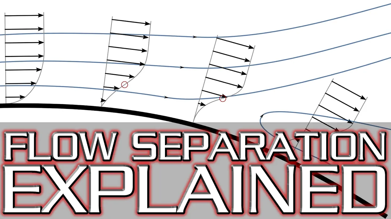
What Causes Stall/Flow Separation? Adverse Pressure Gradient Explained
166.3K
Flow separation and stall occur when an adverse pressure gradient becomes too strong to overcome. The boundary layer is the thin layer of fluid adjacent to a solid surface where velocity decreases from free stream speed to zero at the surface. Under normal conditions, the boundary layer moves in the same direction as the free stream flow. However, when an adverse pressure gradient is sufficiently strong, the pressure forces acting on the boundary layer become greater than the inertial forces trying to maintain forward motion. This causes the boundary layer to reverse direction, creating a recirculation region where flow moves backward against the main flow direction. This phenomenon is called flow separation. When this occurs on a wing, it results in stall—a dramatic loss of lift accompanied by increased drag. The strength of the adverse pressure gradient determines whether the boundary layer remains attached or separates, making gradient management critical for aerodynamic performance.
Click to watch →
Deep Dive
Comparing experimental wind tunnel results with Computational Fluid Dynamics (CFD) simulation data for validation.
![[EN] Seminario web | RWIND 2 - Cálculo de cargas de viento con simulación CFD](https://i.ytimg.com/vi/XGXKJBtTRQ4/maxresdefault.jpg)
[EN] Seminario web | RWIND 2 - Cálculo de cargas de viento con simulación CFD
1K
RWIND enables comparison between CFD results and experimental data from true wind tunnel tests or analytical calculations. Users define comparison points (surface result points) in RFEM, then input experimental pressure values at those locations. Interpolation methods (diffusion for open structures, Gaussian for closed structures) distribute experimental data across surfaces. This allows direct comparison of CFD predictions against empirical measurements.
Click to watch →
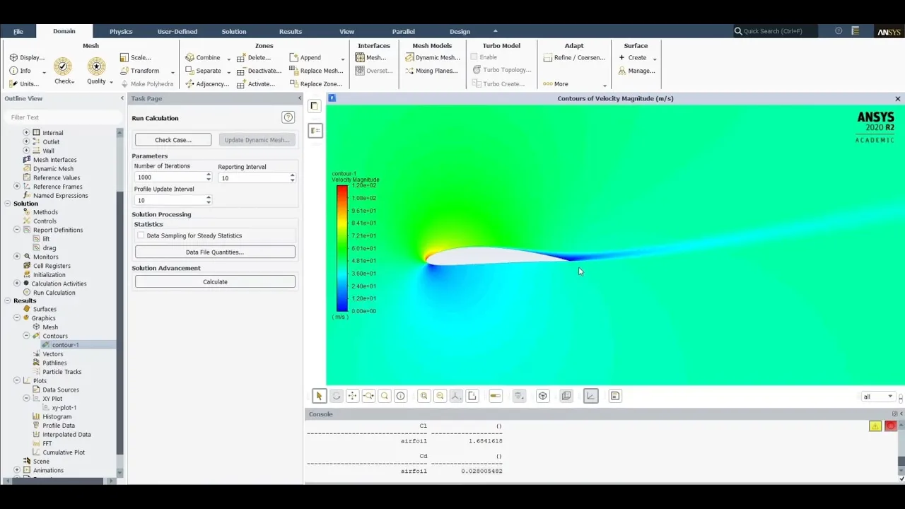
ANSYS Fluent NACA 4412 (or NACA 0012) 2D airfoil CFD Tutorial with Experimental Validation (2025)
283.2K
This section covers the complete CFD solution process including initialization, convergence criteria, and validation against experimental data. Hybrid initialization provides initial conditions for governing equations. Residuals should reach 1e-6-1e-7, but physical monitors (lift and drag coefficients) determine true convergence. Lift converges more reliably than drag due to Newtonian effects versus drag's sensitivity to surface roughness and separation. Expected accuracy of 10-20% deviation from experimental data is considered acceptable given CFD's inherent numerical approximations. Validation compares lift coefficients (NACA 4412 shows ~0.4 at zero degrees) and drag coefficients against sources like NASA Langley Research Center.
Click to watch →

FSAE Aerodynamics (Part 3) | Skill-Lync
296
Wind tunnel testing with pressure sensors (like the GCM truck model with 200 sensors) provides experimental data to validate CFD simulations, ensuring computational results are accurate by comparing them against real-world measurements; this validation process is essential because CFD results cannot be trusted without experimental verification, and simplified models help ensure consistent mesh generation across different CFD solvers for reliable validation studies.
Click to watch →
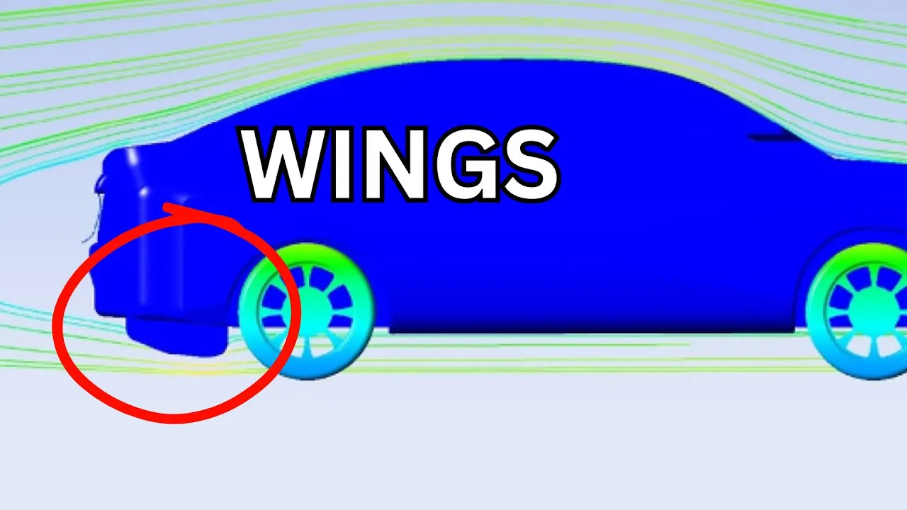
New Wing Car Diffuser Design Podcast 225
3.6K
The study used Fluent U CFD software with RANS equations at 30 m/s free stream velocity (108 km/h). A mesh independence study varied cells from 2M to 32M, achieving 2% drag coefficient variation at 12M cells. Four turbulence models were tested; Realizable k-epsilon was selected for stability. Validation against 1/18th scale wind tunnel testing showed ~10% drag coefficient accuracy with good agreement on major pressure coefficient trends.
Click to watch →
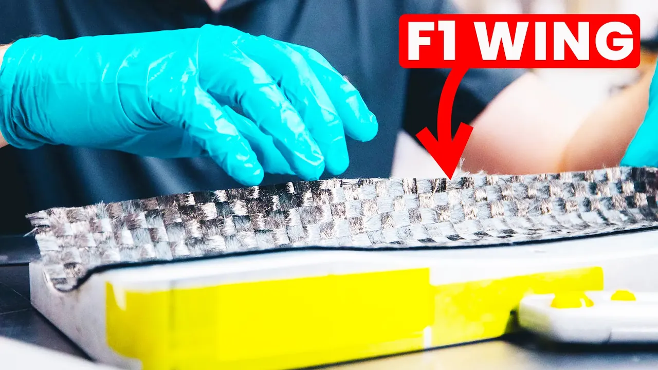
How F1 Wings Are Made
364.1K
While CFD is powerful, it is fundamentally not real because it divides the volume around the car into small blocks, introducing errors at each boundary. Wind tunnel testing uses real air flowing over real models, providing validation of whether designs actually work. However, wind tunnel time is precious and restricted by manufacturers, with only one wind tunnel typically available for all teams to share simultaneously.
Click to watch →
Deep Dive
Investigating the effects of high-lift devices (like flaps and slats) and 3D wing phenomena (such as wingtip vortices and induced drag).

Учебный фильм: Общие основы аэродинамики
99.8K
Wings with lift generate wingtip vortices due to pressure difference between upper and lower surfaces. Air flows from the high-pressure lower surface to the low-pressure upper surface around the wingtips, creating vortices that trail behind the wing. These vortices indicate the presence of lift and cause induced drag. Swept and delta wings experience spanwise flow along the wing surface due to the sweep angle. This flow causes boundary layer separation from the upper surface and formation of a free vortex sheet that sheds from an intermediate point along the span rather than the tip.
Click to watch →

Flying In Ground Effect (Private Pilot Ground Lesson 14)
94.8K
Wingtip vortices form when high-pressure air beneath the wing rushes up to meet low-pressure air on top, creating spiraling air patterns that cause induced drag. Vortex strength depends entirely on angle of attack—higher angles produce larger, stronger vortices and more drag. Wake turbulence poses serious hazards, especially from heavy, clean, and slow aircraft that require higher angles of attack. Flying through these vortices can cause loss of control or flips. To avoid wake turbulence, pilots should fly above preceding aircraft's flight path (vortices sink several hundred feet per minute) and maintain adequate separation.
Click to watch →
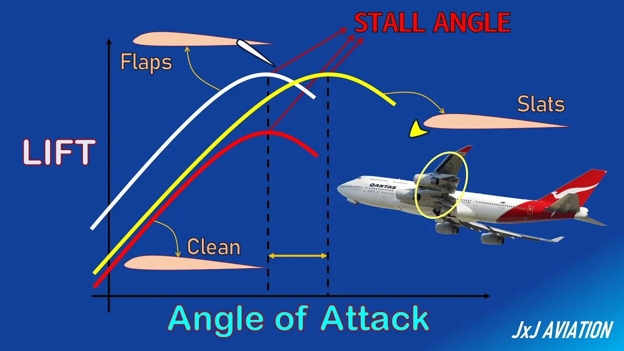
What are High Lift Devices? | Impact of High Lift Devices on an Aircraft Operation | Flaps & Slats
40.9K
High lift devices (flaps and slats) are wing-mounted surfaces that increase lift at low speeds during takeoff and landing; flaps extend from the trailing edge to increase surface area and camber, while slats extend from the leading edge to create slots that delay airflow separation; flaps primarily increase lift without changing the stall angle, whereas slats increase both lift and the maximum achievable angle of attack before stall, allowing safe low-speed flight operations.
Click to watch →

СУПЕРДЖЕТ - Анатомия региональника | аэродинамика и компоновка. Часть 2.
38.6K
Induced drag results from energy dissipated in creating tip vortices at wingtips, where high-pressure lower surface air flows around to the low-pressure upper surface. The Kutta-Joukowski theorem states that dynamic force must be perpendicular to local flow, decomposing into lift (perpendicular) and induced drag (parallel). Induced drag coefficient is proportional to the square of lift coefficient and inversely proportional to aspect ratio. High-aspect-ratio wings minimize induced drag, explaining why long-range transport aircraft employ such designs. Wing-fuselage interference occurs due to boundary layer thickening and adverse pressure gradients, with fuselage area ratio significantly affecting critical Mach number. The SSJ-100 wing features five smoothly connected profiles with thickness decreasing from 13-16% at root to 10-11% at tips, sweep angles decreasing from 27.5° to 5-6°, and twist distribution optimized for cruise performance.
Click to watch →
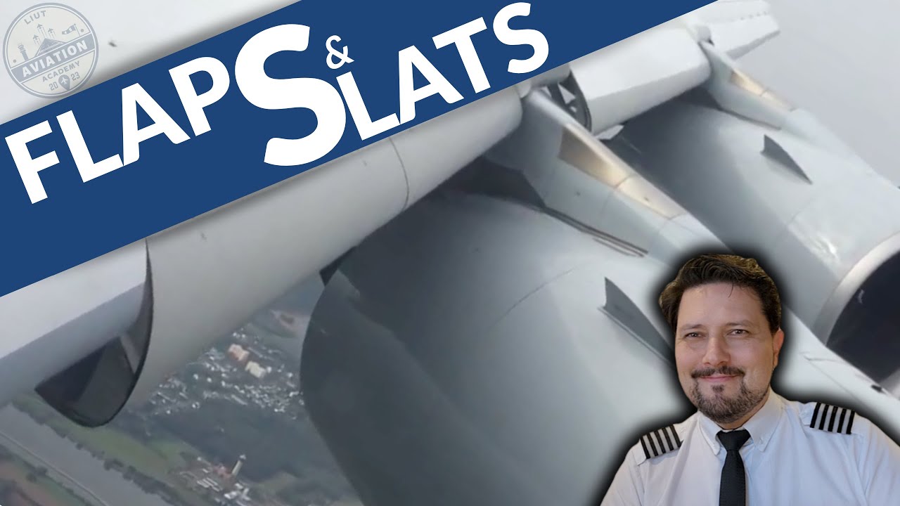
O que são FLAPS e SLATS? A asa “abrindo” no pouso e decolagem!
67K
Flaps and slats are high-lift devices on aircraft wings that enable safe flight at low speeds during takeoff and landing. Flaps, located on the trailing edge, extend backward and downward to increase wing curvature and surface area, generating more lift and drag. Slats, located on the leading edge, create channels that allow high-pressure air from beneath the wing to flow over the top, delaying airflow separation and allowing the wing to operate at higher angles of attack without stalling. These devices are retracted during cruise to reduce drag and improve fuel efficiency.
Click to watch →
Setup Components
Connect Cables
Install Sensors
Ready Control
Set Angle
Setup Components
0:18- 1
Prepare force components and air foil for testing.
- 2
Mount air foil onto standard connections securely.
- 3
Tighten and lock equipment into place.
Computational Fluid Dynamics (CFD) as an Alternative to Physical Wind Tunnel Testing
While physical wind tunnel testing using apparatuses like the Matrix wind tunnel provides valuable empirical data, it is increasingly challenged and complemented by Computational Fluid Dynamics (CFD). Critics of exclusive physical testing point out that wind tunnels suffer from inherent limitations, such as wall interference, support-structure interference, and difficulties in achieving true flight-scale Reynolds numbers. In contrast, CFD offers virtual aerodynamic testing that eliminates these physical constraints. It allows researchers to rapidly iterate aerofoil designs, simulate extreme environmental conditions safely, and visualize flow fields in high resolution across the entire computational domain at a fraction of the operating cost of a physical tunnel. Consequently, modern aerodynamics often prioritizes computational simulation, utilizing wind tunnels primarily for final validation rather than primary design iteration.
Fundamental aerodynamics concepts including lift, drag, and the relationship between velocity and pressure (Bernoulli's principle).
Basic anatomy of an aerofoil, such as chord line, camber, angle of attack, leading edge, and trailing edge.
General wind tunnel operation principles, including flow conditioning, test section velocity, and boundary layer formation.
Introduction to measurement instruments commonly used in aerodynamic testing, such as manometers and force balances.
Calculating and analyzing lift and drag coefficients (Cl and Cd) from raw experimental data.
Utilizing flow visualization techniques (such as smoke wires, tufts, or dye injection) to identify boundary layer separation and aerodynamic stall.
Comparing experimental wind tunnel results with Computational Fluid Dynamics (CFD) simulation data for validation.
Investigating the effects of high-lift devices (like flaps and slats) and 3D wing phenomena (such as wingtip vortices and induced drag).
145 views1likes1:38@MatrixTSLtdOriginal Release: 2023-04-21
I've got my two-force component set up I've got an air foil in ready for testing I would then place that in on its standard connections I will tighten this up lock it in place the standard load knobs that you've seen before I can take the three data cables and I can place them in the Associated ports so I can just place them in here here and here and I can take motor find motor on the two Force component and place that in where I need it to go I can take the lift one find the lift one and so forth that can fit in in there and I can take the last one which is drag load cell and I can place that in there now that's ready to be controlled so I can get myself to control the angle of the airflow which hopefully you can see is spinning as I hold the button down and it's going to go back now to a flatish stage so I'm going to give this a mild angle of attack something like there we go so I'm about there
Up Next
12:46
How to Calculate Lift: Lift Coefficient and Angle of Attack
@AliyaBurkit
60K views•2020-05-28

30:32
Ultrasonic Transducers: Resonant Frequency Measurement and Horn Design
@imajeenyus42
229.9K views•2017-02-22

54:16
Polymer Environmental Degradation: Mechanisms & Stabilization
@iit
1.8K views•2012-07-10

33:39
How a Student's Question Saved a NYC Skyscraper from Collapse
@veritasium
22.8M views•2025-04-26
Related Study Plans & Knowledge Roadmaps
Structured learning paths in Engineering
engineering
Building Acoustic Levitators: Physics & Arduino
01The Physics of Sound and Standing Waves
02Piezoelectric Transducers and H-Bridge Drivers
03Arduino Programming: Generating 40 kHz Signals
+ 2 more learning modules
14h5 modules
Explore Roadmap
engineering
Building Peltier Cloud Chambers: Particle Tracks
01Cosmic Rays & Cloud Chamber Physics
02Thermoelectric Cooling (TEC) Fundamentals
03Custom Liquid-Cooling Loop Design
+ 2 more learning modules
18h5 modules
Explore Roadmap
engineering
Yagi-Uda Antennas: Modeling, Build & VNA Test
01Introduction to RF and Antenna Fundamentals
02Yagi-Uda Antenna Design Principles
03Antenna Modeling and Simulation in 4NEC2
+ 2 more learning modules
18h5 modules
Explore Roadmap
engineering
ECG Monitor Design: Op-Amps, Filters & Noise
01Electronics & Breadboard Basics
02Op-Amps and Instrumentation Amplifiers
03Bioelectricity and ECG Fundamentals
+ 2 more learning modules
18h5 modules
Explore Roadmap