


![[Teoría descriptiva conjuntos] 38. Sigma-álgebra de Borel, funciones Borel](https://i.ytimg.com/vi/6fojakSjogE/maxresdefault.jpg)







![[s3 | 2025] Математический анализ, Семенова О.Л., лекция 30](https://i.ytimg.com/vi/hc35NooDRoo/maxresdefault.jpg)
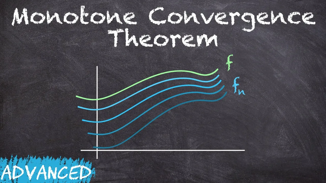


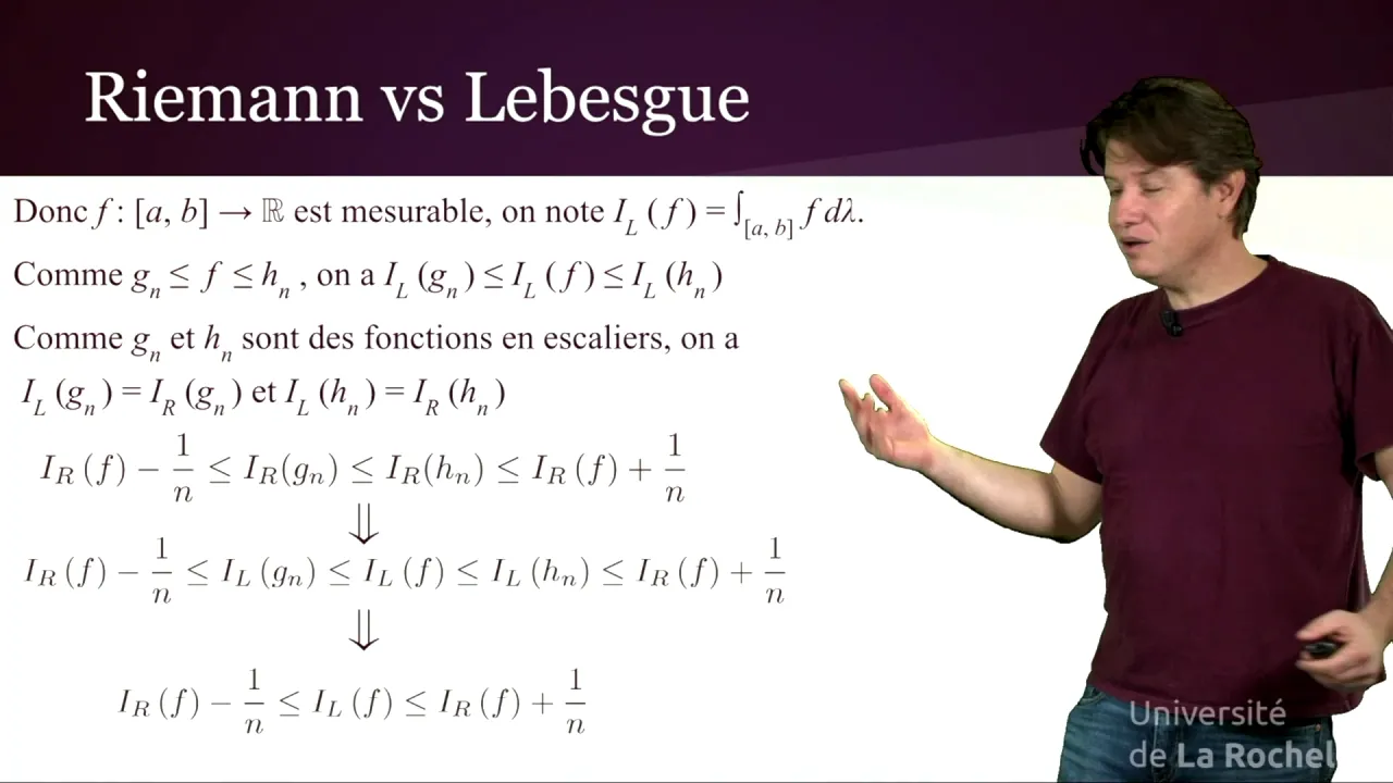
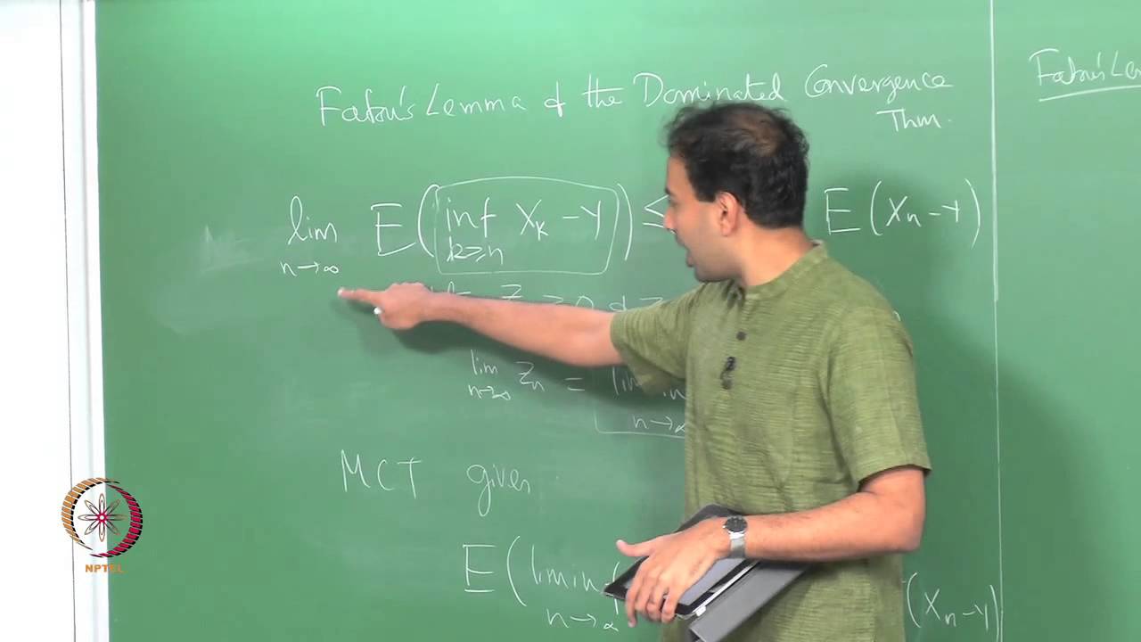

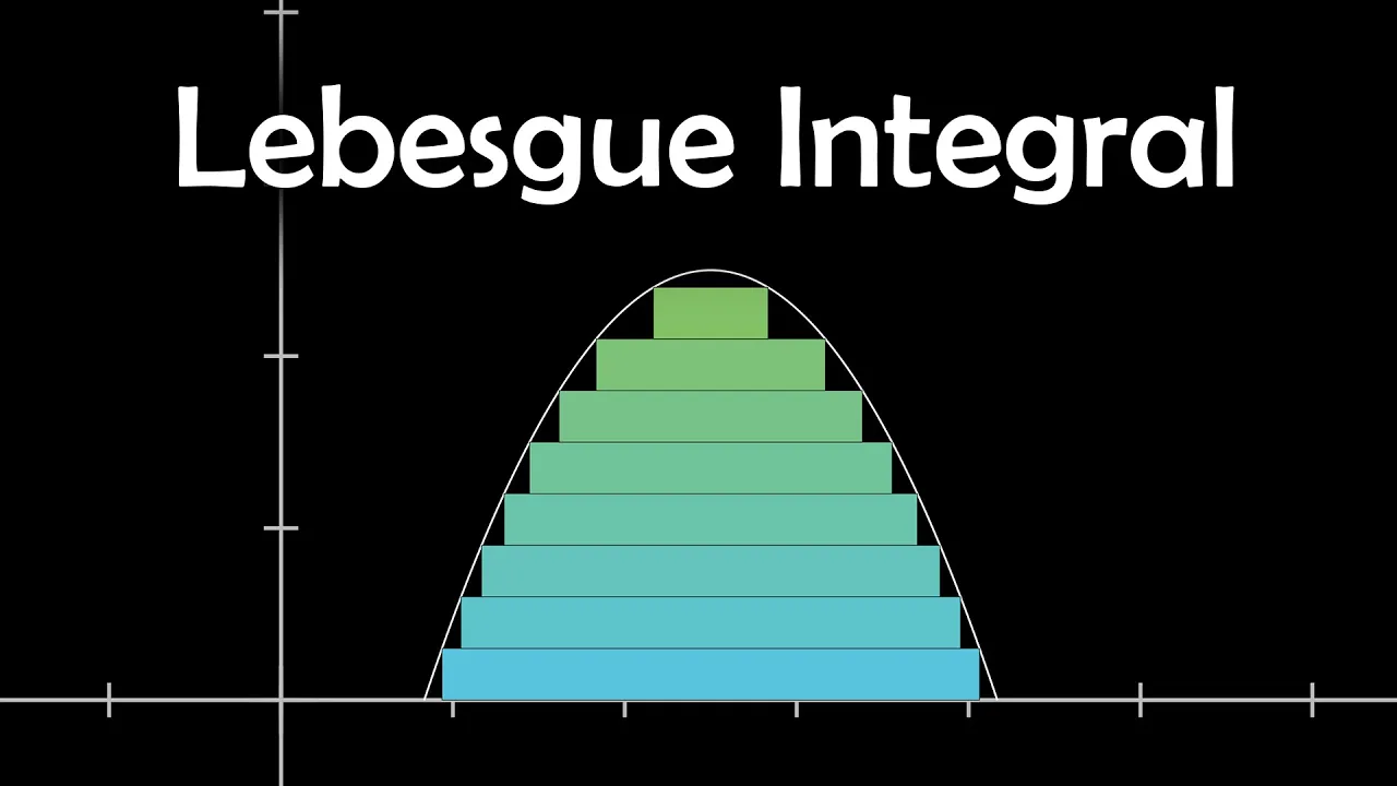
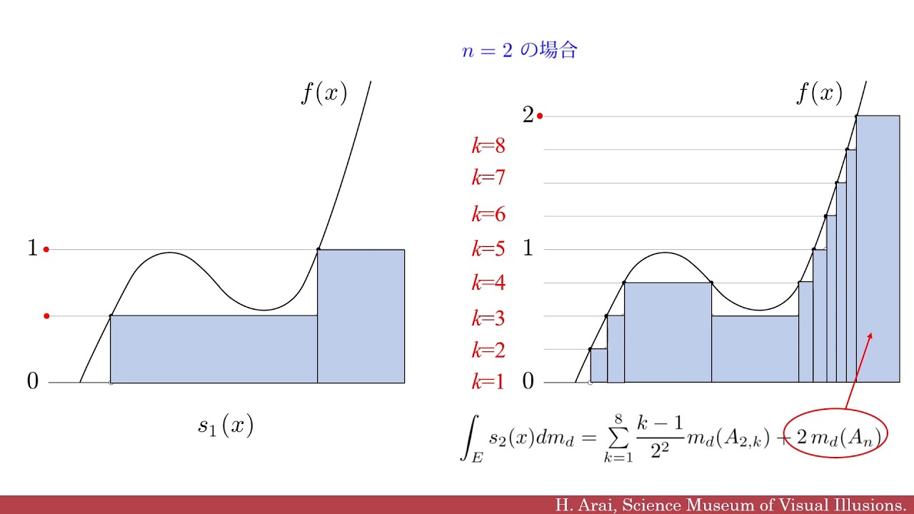
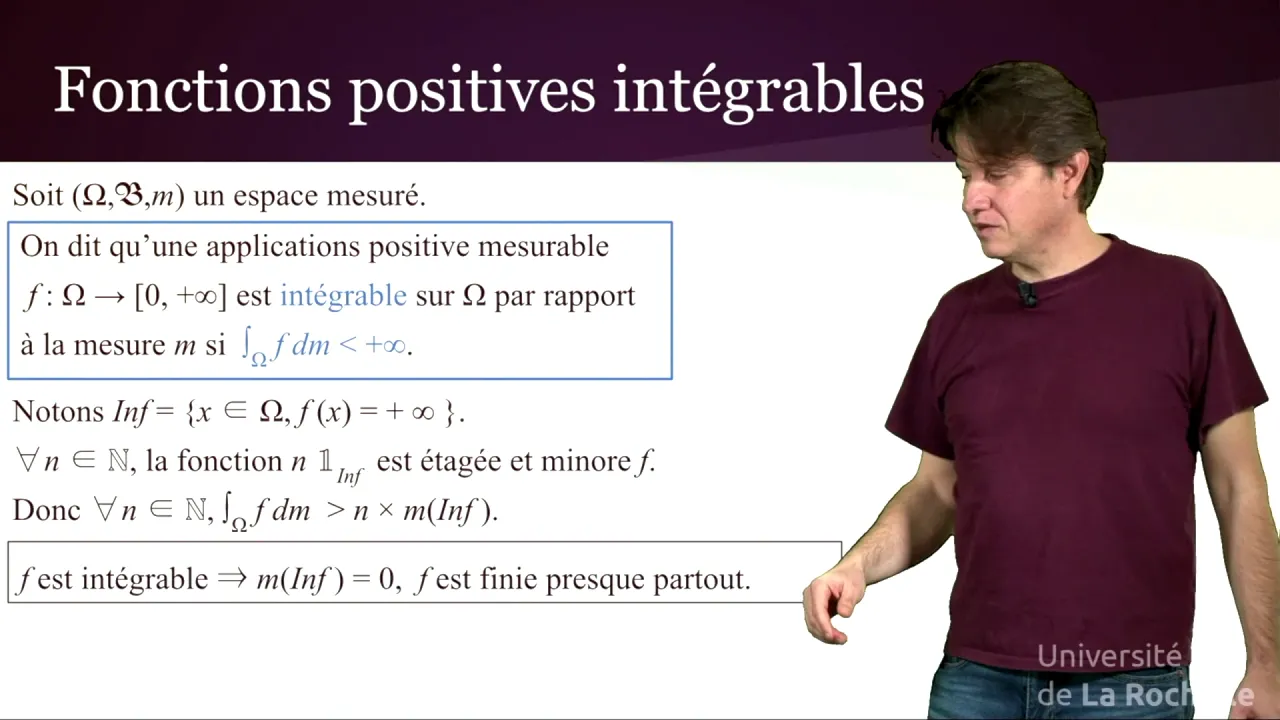
The Lebesgue integral for non-negative measurable functions is defined as the supremum of integrals of simple functions that lie below the given function; specifically, for a non-negative measurable function f, the integral ∫f dμ is the supremum of all ∫h dμ where h is a simple function satisfying h(x) ≤ f(x) for all x in X, and this definition extends the integral from simple functions (which are linear combinations of characteristic functions of measurable sets) to general measurable maps by approximating them with increasingly refined simple functions.
Measure Theory 6: Lebesgue Integral of Simple Functions
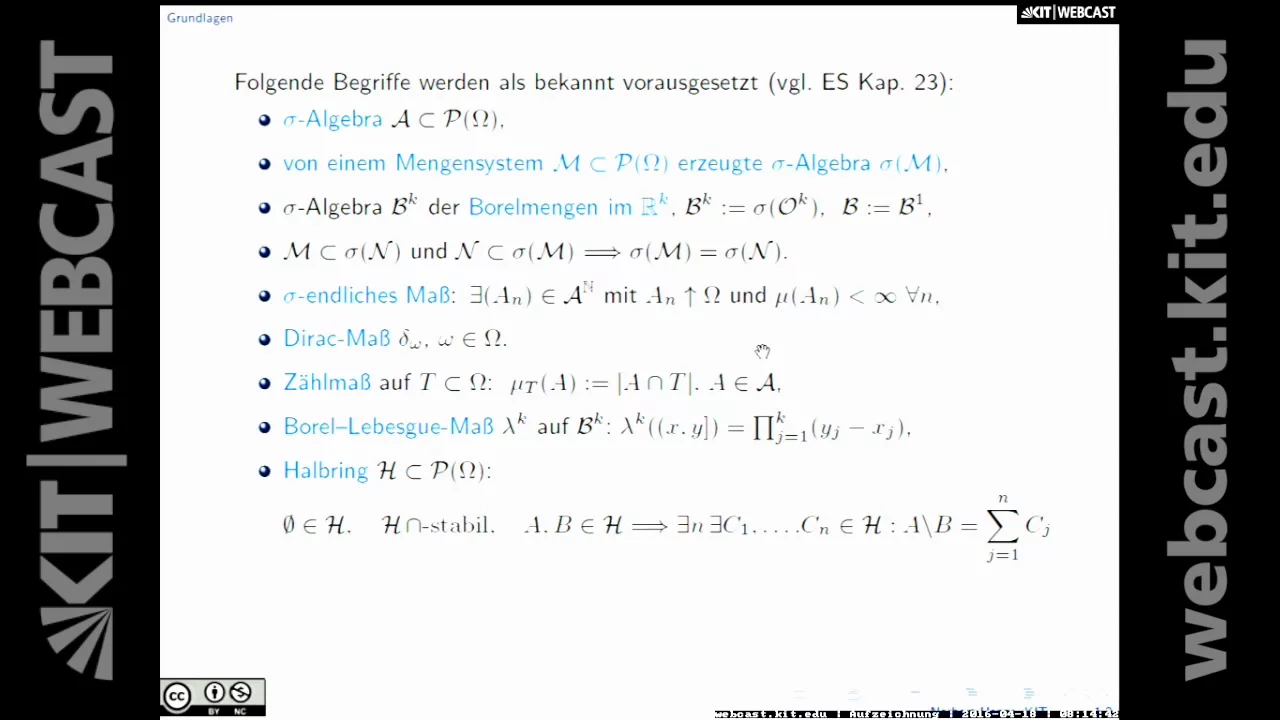
Added:Definition of a measure space, including sigma-algebras and measurable sets.
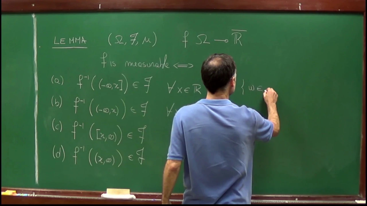
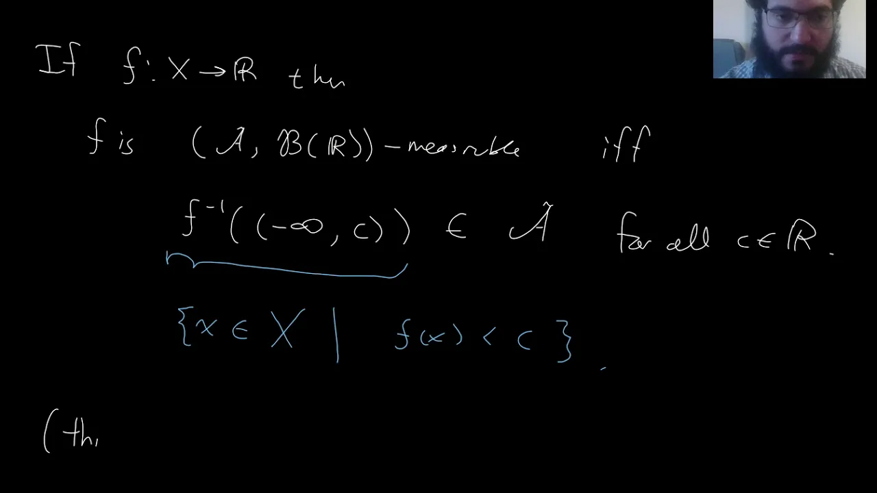
Concept of measurable functions and their properties (such as preimages of Borel sets).
Definition and mathematical representation of simple functions (finite linear combinations of indicator functions of measurable sets).
Basic understanding of the Riemann integral and its limitations with highly discontinuous functions.
Extending the definition of the Lebesgue integral to all non-negative measurable functions using supreme limits of simple functions.
The Monotone Convergence Theorem (MCT) and its role in exchanging limits and integrals.
Defining the general Lebesgue integral for functions with both positive and negative parts, leading to the definition of L^1 space.
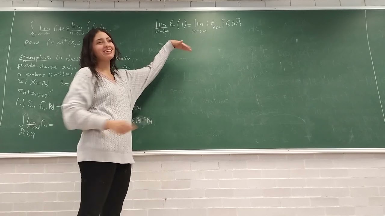
Fatou's Lemma and the Dominated Convergence Theorem (DCT), which provide powerful tools for limit operations under the integral sign.
141.9K views2.8Klikes23:01Original Release: 2019-09-29
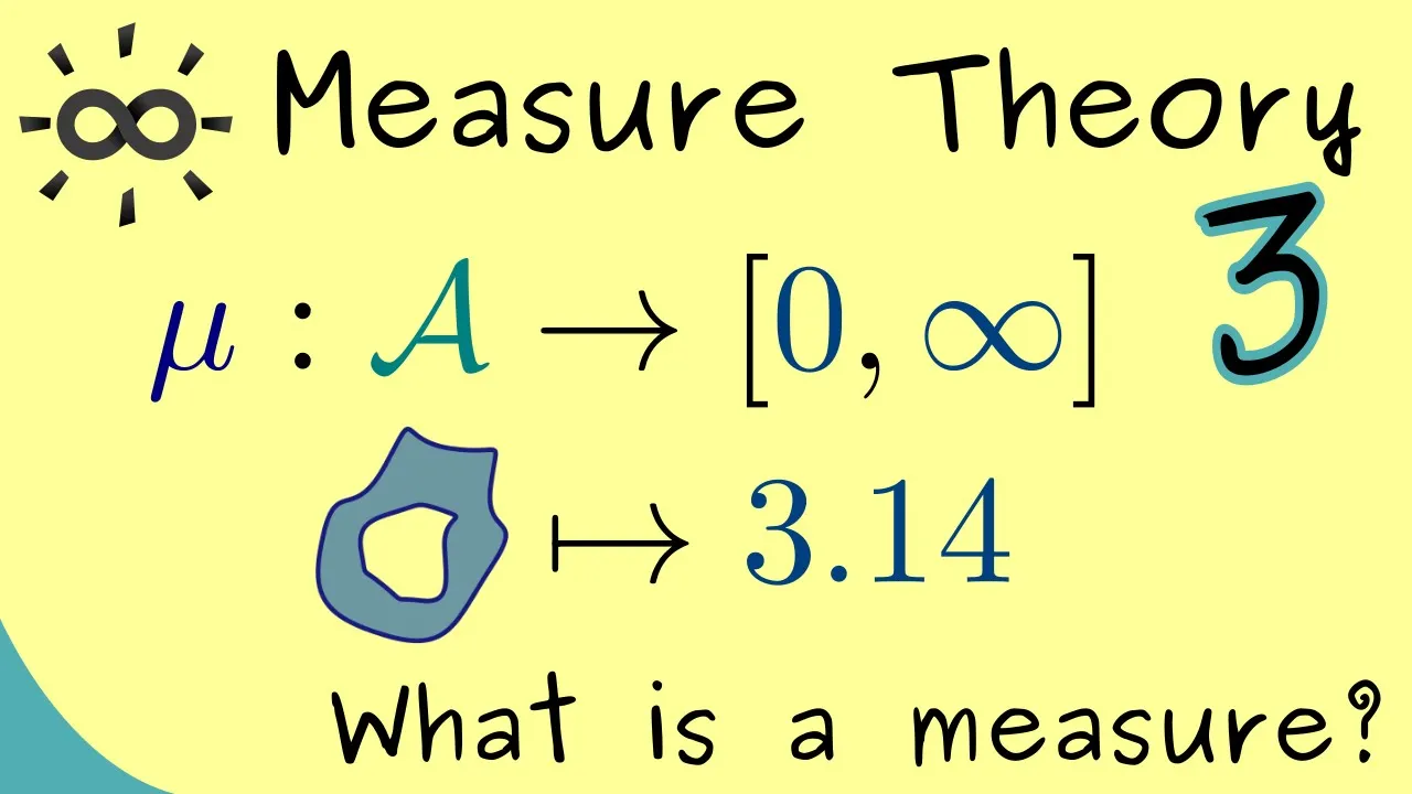
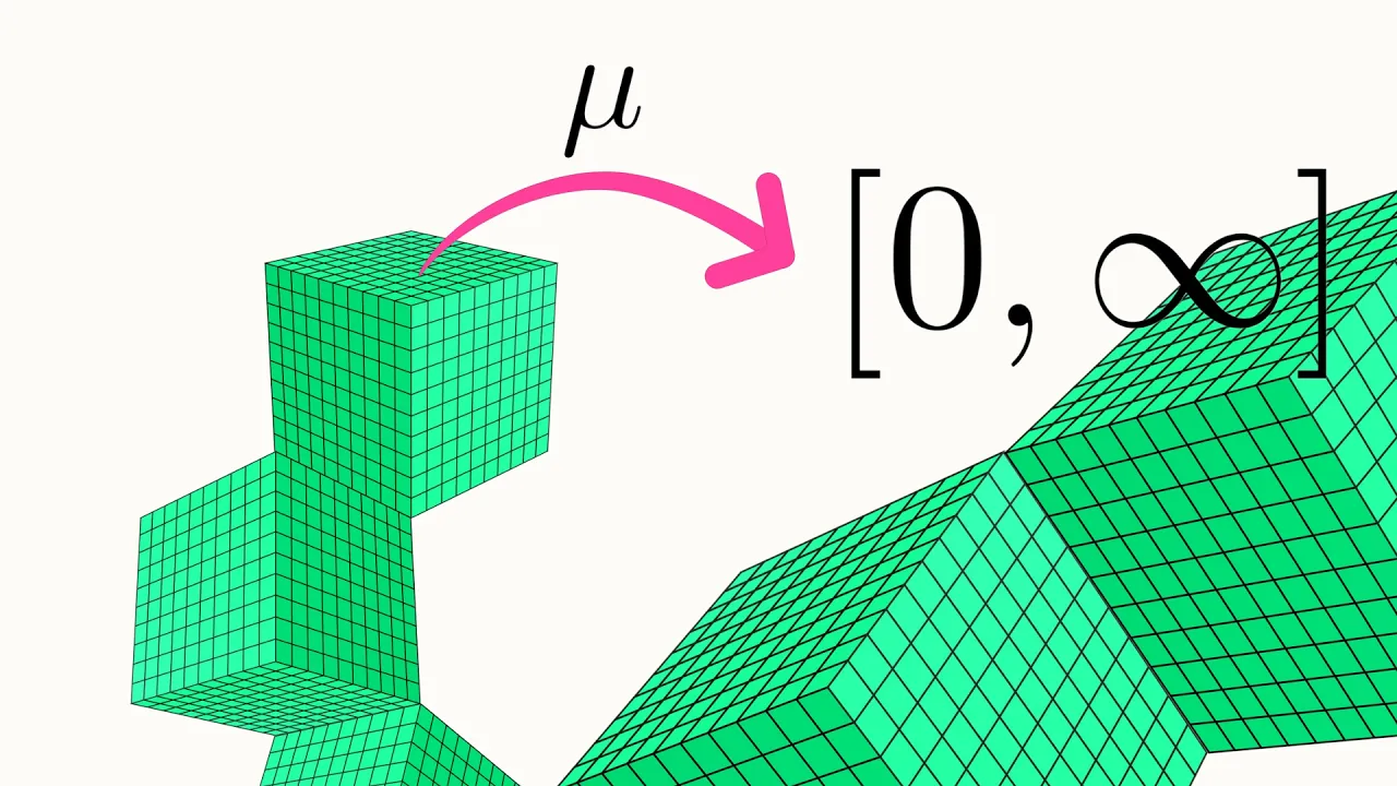
hello and welcome back first let me thank all the nice people that support this channel on steady and now let's continue with measure Theory namely with part 6 and we will finally talk about the lebesgue integral but first about the lebesgue integral of so called step functions so we will learn how to integrate functions that are defined on an abstract measure space as a short recap a measure space is nothing more than a Tribble there we have set X Sigma H bar a and also a measure mu this means that X could be any set but a is a special collection of subsets of X and the third ingredient the measure move itself is indeed a map where the domain is the Sigma for a and the codomain is the interval included 0 and also included the symbol infinity now with respect to this abstract measure space we want to integrate some special functions indeed what we need are measurable maps defined in the last video I will use the letter F for such maps that start with X and go into the real number line now you should not forget that we have a Sigma algebra on the left namely a and also Sigma J on the right and there we have the Bou L Sigma algebra also we call that measurable means that all the pre images from elements from the Sigma algebra here lie in the Sigma algebra a in other words three image off I said E is in a for although L sets E ok so these are the functions where we want to be able to integrate them you the end however at the moment they might be too complicated so we start with functions that we already know for example we already know that the characteristic function is a measurable map if we choose a measurable set this means a nice in the Sigma H bar we already know how to sketch this function if we have our abstract X here on the line and maybe this is set a so these two things together I then we can sketch the graph of our characteristic function it will be zero here and as to where you want we had a set a lies so here it would be 1 and here also 0 and they also do for visualization of the integral it's always good to see the integral as the area below the graph and the x-axis here this would mean we look at this area here and the area here and because the value of the function is just 1 it doesn't matter how abstract this whole measure space is this area should be exactly the same as the volume the measure of the set a or in other words a meaningful integral notion and maybe let's call it just by capital I of this characteristic function should always fulfill that this integral is the measure of the set a now we have a new symbol on the left eye of a function so you should read this indeed as in definition this means now you know how to integrate characteristic functions in fact there are other functions where we can define the integral also in such a simple way and these are called simple functions they are also a lot of other names that one uses for simple functions for example step functions as I did in the title of this video and also staircase functions and also our names and you see the name might not be important you just have to know what such simple functions are in short a simple function f is just a linear combination of such characteristic functions this means you can write f of X as the sum now we start with 1 and go to a fixed n and where we have numbers C I and characteristic functions corresponding to some measurable set a I in other words a function f is called simple if you can find measurable sets a 1 to a n and real numbers C 1 to C n such that you can write the function in this form because we know that the characteristic functions are measurable and also sums of measure both maps are also measurable we also know that the simple function is therefore measurable also here I would say to get some visualization let's sketch the graph of such a simple function this is the same as before so we have X here and our hero and maybe here now we have set a 1 and here set a 2 and let's choose the split set a 3 here and for these sets we can now choose some constant C I hence we have for the graph of the function some value here over a 1 and not I will you over a 2 here and maybe a lower one here for F we and outside of these sets we are just at zero if we now go back to our Liz Asian of the integral we know it's given by rectangles for example here we have two rectangle with length given by a 1 and the height given by C 1 therefore this rectangle here just represents the part of the integral that is given by C 1 times the measure of a 1 and the contribution for in the curl given by the set a 2 is just this rectangle here and of course now given by C 2 times the measure of a 2 and then the last part is coming from a free which consists of three parts but in the sum of course this is also C 3 times the measure of a 3 and now you should see that we just have to add up all these contributions to get the full integral to get the full area in this picture hence again for meaningful integral definition we need a sum of all these parts so I of F is then given by a sum and there I have the same CI as before but now not the characteristic function but the corresponding measures of the sets and indeed this will be our integral for simple functions in the end however at the moment you should see immediately one problem of this definition what happens if we have a set with volume infinity so that this number here is the symbol infinity there we could have for example 3 as the C times infinity maybe that's not a problem for you because it's just infinity itself again but then what happens if the next C here is minus 2 and it measures also infinity and of course this is not simply just 1 infinity is not defined at the moment in fact we have a problem with the definition in general in order to solve this problem they are essentially two ways one can go now on the one hand one can restrict oneself to such simple functions where the corresponding a eyes only have finite measure obviously then there's no problem with such infinities because there's no simple infinity involved in the whole Sun and on the other hand one can demand that these constants have to be positive then there might be infinity in the Sun but only with the same sign and then of course we don't have a problem adding up positive infinities and exactly this second possibility is the way I want to go here now finally we can put the integral into a definition for this we will consider now just functions defined on X and as before there should be step or simple functions moreover we want now to consider only the positive ones or more concretely the non-negative ones the whole set of such functions is now denoted by a curved s where I put in a plus and this as plus is now almost a vector space in the sense that we can add functions as we want but we can't scale them as we want because only positive scalars are allowed otherwise we would leave this space so you should imagine this as a half space if we go now back to our definition of a simple functions you immediately recognize that this representation here is not unique for the function f for example we could split to set a two into two parts and then we have one term in addition in the sum here but it does not change the function f itself so the graph looks still the same just this is different therefore another description which is independent of this representation for simple function would be I have a measurable function and it only takes finitely many values in this case I can always find such a representation here the idea is now always choose a suitable we presentation for your simple function f in our case here if F comes from our s plus then choose the representation as always so we can write it as a sum but now where the sea-ice are also non-negative of course if the function is non negative then we can always choose such a representation and now it's very easy to define the lebesgue integral so this is our new notion and of course often we will ignore the Lebec and just speak off the integral now because this is the integral we define here and to be more concrete we also would say with respect to our given measure mu and this integral is now given as we already know and also denoted by I of F where we just add up the measures of the sets a I where we scale them what so by the sea-ice so we have C I times the measure of a I and because the CI are non-negative and the measure itself is non-negative or the worst case just infinity we know this integral is now also in interval 0 to infinity where we include both parts 1 fact I can give you immediately this definition for integral is a well-defined object this means that it does not depend on the chosen representation for a simple function f so if you choose another we presentation with this property you get the same number out maybe this is a thing you could try to prove however of course the visualization should be the important thing so it does not matter how you split up these rectangles here yet the sum or the sum of the areas should be always the same no matter how you split up these sets here on the x-axis or you split up the Z values on the y-axis in other words it makes sense that this integral here is indeed the defined and finally I can give you the usual notation one uses for the integral of course an integral sign we put the set X here then comes the function f and then the measure mu by D mu sometimes also a variable is needed and the notation looks almost the same so you just include a variable name for the function so a lowercase X here and then T mu X so this is the lebesgue integral for step or simple functions the idea is now that we expand this definition such that we can also integrate more complicated functions but before we do that let's first look at some properties this integral has firstly it is almost linear I already told you we almost have a vector space for OS + + this sense it's linear we just have to restrict the scanners to non-negative numbers and then we can pull out the addition sign and also the scalars hence this equality holds for all simple functions F G and for all scalars alpha beta greater or equal than zero and of course this immediately comes from this sum here also by using a we can now show that if we have a step function or simple function that always bigger than another one so we have F less or equal than G then also the area between the curve and the x-axis should be bigger for G than for F and of course this what the integral tells us so I of F is also less or equal than I of G and this is what one calls monotonicity in fact this monotonic behavior is what we now can use to expand our definition to general measurable maps in order to get a visualization let's sketch again a graph now this is the graph of some measurable map which is not a simple function as you can see now the integral should be now again we presented by the area below the graph and the x-axis however we only have this notion for the moment for the simple functions and as you know by now a simple function has only finitely many values and this blue graph here shows you they are infinitely many values the whole idea of the back integration is now to approximate the function by finitely many values so I just choose some values here on the y axis such that the whole curve is in some sense covered and now the idea is to define a suitable simple function therefore maybe I choose this interval here and look what happens to the values of the function they are and now you see we have two parts that are mapped to this interval here for the x-axis this looks like this so we have this part here that ends here and we have this part that starts here and also ends here this means we have one part of our set here and the other part here and of course this should be our set that we usually call a I so this is just one a I and the corresponding see you find now here so this would be our CI so I shows the lower part of the interval because then our step function is also below the graph of the function so this would be the value of our step function here and now you see all the other values on the y-axis give us the other CIS and also the corresponding a is therefore with this decomposition of the y-axis we get out the user step function maybe have our CI stare and the so defined a is where we have to know the characteristic function here so this is a new simple function which I should call H now and the important part is that H itself lies always below F so always below the graph that is blue here therefore if we want to contain the monotonicity in the general integral we now have an estimate for the real integral value of the function f we know that the integral of this step function is smaller than the real integral and this gives now rise to the following definition hence we choose a positive or beta and non-negative function f that is defined on our measure space X and of course it should be measurable and now for each decomposition of the y-axis we can choose such a step function or a simple function age that lies point wisely below the graph of the function f itself and if we use the function H out of the step function that are positive or non-negative so as plus we know we can look at the integral of this age what we have has done a whole set of integral values where the only condition is that our step function is always below the real function f the general idea is now okay so this integral value for the step function is always smaller than the actual integral value for the function f and we should get closer and closer to this value if you choose a finer and finer decomposition of the y axis so we approximate something with the set here and of course this should be the supremum of the set in fact this is what we choose as the definition of the integral for a function f so we have F T mu and also this is our middle space X so the integral of a non-negative measurable map F is given by the supreme 'm of all integral values for step functions that lie below the function f and that is now the definition of the lebesgue integral and we also see this is well defined the supremum of a set in the real numbers always exists in the worst case it would be infinity therefore in addition we also have another definition f is called mu into global if the integral is finite so it's not the symbol infinity and there you have it this is our result for today the lebesgue integral in complete generality because you see the only thing we needed here was a measure space X so we only need to know how to measure the volumes of these sets on the x-axis however what we used is that we map into the real numbers so indeed here we have are on the y-axis therefore we can do this decomposition we can't do this decomposition in the x-axis because there is no orders nothing more than just the measure but on the y-axis we can do it now it should always keep in mind the lebesgue in the curl is just defined with a supremum where use simple functions to define the integral first so this was a long video today and I hope you learned something here of course we had to define a lot of stuff but in the end you saw it is just a simple function where we can write down the integral immediately and then the general integral is just an approximation concept in the next video I will continue with the lebesgue integral and also write down a lot of properties we have for it and afterwards you will finally see why the lebesgue integral is so powerful then I have a nice day and see you next time bye
Up Next

26:23
Lebesgue Integral Explained | Measure Theory & Integration Overview
@drpeyam
109.8K views•2018-02-09

4:43
Elliptic Curve Cryptography Explained: ECC, ECDSA, ECDH
@PracticalNetworking
28.5K views•2024-10-21
8:22
Laurent Series Explained | Complex Analysis
@brightsideofmaths
52.4K views•2022-04-06

6:00
The Mathematical Impossibility of Accurate World Maps
@Vox
23.3M views•2016-12-02
Related Study Plans & Knowledge Roadmaps
Structured learning paths in Mathematics
mathematics
Tensor Calculus: Vectors to Riemann Curvature
01Mathematical Foundations: Linear Algebra & Calculus
02Covectors, Dual Spaces, and Tensor Basics
03The Metric Tensor and Index Gymnastics
+ 2 more learning modules
40h5 modules
Explore Roadmap
mathematics
Gödel's Incompleteness: Logic, Proofs & Limits
01Introduction to Formal Systems & Hilbert's Dream
02Set Theory, Cardinality, and Cantor's Diagonal Argument
03Arithmetization and Gödel Numbering
+ 2 more learning modules
14h5 modules
Explore Roadmap
mathematics
Galois Theory: Fields, Groups & Solvability
01Foundations of Abstract Algebra: Groups & Fields
02Polynomials & Field Extensions
03Splitting Fields & Symmetries
+ 2 more learning modules
24h5 modules
Explore Roadmap
mathematics
Non-Euclidean Geometry: Models & Geodesics
01Euclid's Fifth Postulate and the Birth of New Geometries
02Hyperbolic Space and the Poincaré Disk Model
03Geodesics: Defining Straight Lines in Curved Spaces
+ 2 more learning modules
15h5 modules
Explore Roadmap