Legendre Transformation and Thermodynamic Potentials

[00:00:02][Music] Okay. So we have introduced uh new quantities while talking about the spontaneity of reactions. For example, we talked about helmo free energy a as u minus ts and gives free energy g as h minus ts and also u u also h enthalpy as u plus pv. We talked about enthalpy before but uh in the context of spontaneity we talked about enthalpy um in the last lecture. Now we are going to tell you that uh these uh different things like enthalpy helmo free energy gives free energy they are not some quantities just for spontaneity itself they have a deeper connections with the thermodynamics because they are all thermodynamic potentials. So how do we understand that? So in order to understand why they are thermodynamic potentials and why they're important because again if they are they are criteria for spontaneity means of course they have some role to play in determining the the change of matter which direction it will go and all. So we are going to talk to we we're going to show you that how these quantities arrive and that is typically known as legendra transformation. So the uh the reason that legendary transformation is important or it came up because if you look at the fundamental equation So fundamental equation in U depends on S, V and N. In fundamental equation of U which is called energy fundamental equation.

[00:02:11]There is also corresponding entropy fundamental equation where S is a function of U, V and N. So if you see the fundamental equation U depends on S, V and N all are extensive variables and it is not always easy to measure the extensive variables. Often we want to have quantities uh parameters that uh depends on intensive variables like temperature, pressure and things like that. and because they're easy to measure in experiment. So therefore uh it would be good to have a function that depends on intensive variables. However you know that if we do that if we take the derivative of the function for example if I take du by ds as you as you saw um earlier at a constant at a constant vn it'll give you the intensive variable temperature. Now in that case we are losing information. I can give you an example of a one-dimensional function. Let's say y depends on x and let's say this is the function that we're talking about and you know the derivative of the function which means slope I can obtain at any any point by let's say you know uh calculating uh slope of the function p which is let's say defined by dy by dx. So if you see this particular function slope then this P is not really an unique quantity because P can be obtained. So P is unique quantity but it can be obtained from multiple values of Y. For example, if Y is expressed as Y + C or let's say yeah Y + C. So let's say a function of another function of y1 x depends on yx + c. In that case d y1 by del x is same as d y by d x. So p will be same in the cases of so many different functions which are created by adding some constant value. So therefore P will be same for a series of functions. So now if I draw a series of function like this which are all like parallel and shifted by C then all of them will give the same P. So therefore whenever we take the derivative we are no longer going to get the same fundamental equation because remember the fundamental equation has all the information. However, derivative of the fundamental equations which we call as equation of state that does not have all the informations because we are projecting onto a particular uh lesser dimension. For example, what I mentioned here that many of many functions will give the same value of p at that. So therefore the concept of legendary transformation is that you want to keep the same information. However, you want to express uh same uh information that is there in the function yx by something else.

[00:05:47]So for example, so let's say this is my y and this is my x and all the different points represent for a given value of x a particular value of y or or all possible values of x and y is our particular graph and in that this graph represent that for a given value of x for a given value of x what is the value of y for a given value of x what is the value of y For a given value of x what is the value of y? So for every value of x there is a particular value of y and that is what the graph is and this graph let's say contains information about the system of you know thermodynamic system. So in that case if I just take the slope as you see that it will not be possible to exactly determine the uh all the information about the system. However let's say instead of slope if we also calculate one more quantity and that is intercept of the function. So in that case this particular point XY let's say I call it XY1 X1 Y1 will give a particular value of P1 slope and a particular value of intercept let's call it S1. So every point xy1 y1 on the graph will correspond to a particular point let's say this point is x2 y2 will give us a particular point of p2 and s2. So therefore we can map a function xy to cip and that is what the legendary transformation is. So given a graph xy where for every value of x we have some value of y we can always have all the informations contained in the graph be represented by another pair of points s and p. So for every value of this thing we'll get that and therefore we are not we are not compromising on any information as soon as we put the s it will be no longer same as uh for all possible parallel lines because as you can see in this particular case if I have a slope here it will have a particular intercept and this slope will have a different intercept. So if we talk about only slope they may be similar but intercepts will be different for these parallel lines. Therefore keeping both the slope and the intercept we are going to map the complete information from xy point to a cip point. And as you know the P as you have as I have discussed that P is an intensive variable now because it comes as a derivative and S is uh now a function of that intensive variable P. So therefore we can represent a thermodynamic function yx where x is an extensive variable to be cast into another function where that function is a function of intensive variable. So this is intensive and this is extensive. And reason is just that we want to express a function in terms of intensive variable for our convenience because it is convenient to measure temperature. You you know that right the you know several several ways to measure temperature but there is no way to measure the entropy of a system. So therefore if you cannot measure the entropy of a system we cannot get the value of U. But if we cuss the same information into something else where we can measure temperature and get the information about that then we get the information about the thermodynamic system much more easily.

[00:09:43]So that is the reason of converting this uh one one set of pairs of points to another set of pairs of points. Now how do we do that? It is actually extremely very simple. So for example we know the definition of P. P is a slope. Slope means you know the difference in Y. I'm talking about two points. One point is xy on the graph and another point is 0 and s because as you know s is the intercept right? So intercept mean meaning the value of y at x=0. So value of y so this is also x y points but value of y at x=0 is nothing but s because that is the intercept of the function. So this is let's say for example this is the value of y at value of x equal to0. So therefore I'm taking two points one point is this particular point and another point is any any of the points that is mentioned here xy. So then I'm talking about d uh slope is nothing but dy by dx which is delta y by delta x. So I'm talking about uh the difference between y - 0 divided by y - s divided by x - 0. So that's the definition of slope. So then automatically what we get is XP is Y - S and what we get from there is S is Y - XP which is if I write it a little bit in a nicer way P is nothing but slope of the function. So dy by D X into X. So this is for one-dimensional function. So you can see that for multi-dimensional function let's say if if it um depends on more than one variable let's say our y depends on more than one variable then we have to use a sub sub subscript for that so so that we can talk about only slope in one particular variable we are going to show you immediately right now so this is what the legender transformation is this is what called legendra transformation so you see that by doing The legendary transformation we have not compromised anything. We have got all the informations at the same time we have cursed our function uh uh which which was dependent on extensive variable to now a function which depends on intensive variable. Now we will do that and we'll show you that how we can get that. So let's talk about our y which was a function of x as u as a function of s v and n. So this is our thermodynamic uh fundamental equation right. So now we're going to write a function s which is u minus derivative of u with respect to x. So del u by del s. And since it depends on multiple variables I said that we have to use the other variables as constant and then we have to just multiply with s and you know what is du by ds at a constant v and n right? That is nothing but t. So u minus ts and u minus ts we already defined as a. So you see we got homogeneous energy just by we we name it as homogene energy but this a is nothing but legendary transformation of u. Now you you know that we are going from yx to cip p is a slope. So here this is the slope right. So therefore it will depend on t and since we have not changed the variable v it will depend on v and n. So now a depends on tv and n.

[00:13:34]So so since u was a thermodynamic potential a is also a thermodynamic potential. So let us now do another transformation which a different variable. Now we do u minus now we are going to do with respect to v. So d u by dv v at a constant s and n v and what does what does that give us? U now minus du by dv you know is plus right plus p u + pv and we have defined earlier named it as h. And what does it depend on? It will depend on the slope which is p and rest of the variables will be constant which is s and n. So h is a function of sn and we call that as enthalpy. Now we are going to do one more s as both the variables. So we we do now regener transformation on both the variables. So d u by del s at a constant v and n s minus d u by delv at a constant s and n v which gives us u - t s minus plus pv and u plus p v is h minus d s and that is nothing but g and it will depend on which are the slopes t and p so t and p and n did was not change. So n is also there. So this is called gives free energy or we name it as gives free energy. So now so you see that from one fundamental equation where u is function of extensive variables we have arrived at three new fundamental equations and three new thermodynamic potentials where now the variables got changed to from extensive variable to intensive variable. For example, you can see G is function of two intensive variables and and H here is function of one intensive variable because only one we changed and uh helmo free energy is function of one intensive variable because one only we changed but G is function of two intensive variables only one extensive variable that is N. So you see now we call this u particular um thermodynamic potentials like a h and uh g are nothing but abdar of the same god because it it only appears that they are there for they are there with a different appearance however with the same identity underlying information contained in this particular thermodynamic potentials uh is always same whether or not we uh we write them in a different way.

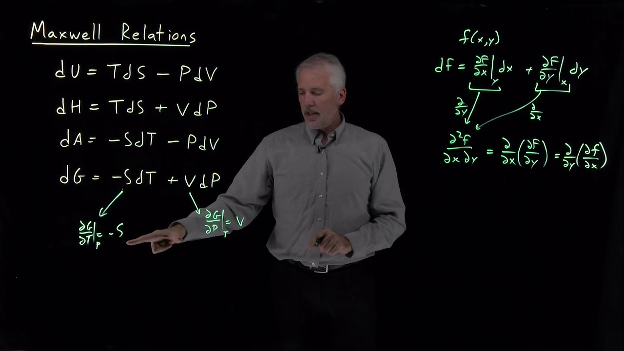
[00:16:24]So so once we get that now we will summarize again our all thermodynamic potentials. So u is a function of s v and n and we have seen that d u as du by del s v n d s plus d u by delv sn dv and we are not talking about n now so that is tds minus pdv okay so Now h is a function of s p and n and therefore you can write dh as delh by del s pn d s plus delh by delp p s and n dp which is delh by d ss constant p and n is nothing but t ds and delh by delp is v. So tds plus v dp right. So we we also know that because you know h is equal to u plus p v. So delh is del u + p dv plus v dp and du plus uh d uh as you know that du equal to dq + dw which is tds minus p dv. So therefore, du plus p dv is nothing but tds. TDS plus vdp and that's what we got here. And we know that delh by d s is t and del h by delp is v.

[00:18:13]Similarly, we got a as t v and n which you expand as da d a by del t at a constant vn dt plus d a by delv at a constant tn dv. Remember we are not doing the n part but otherwise it's fine. Now what is this quantity? In order to understand that we have to expand that as u minus ts. So da is du minus dds minus s dt.

[00:18:46]And what is du minus dds? It is nothing but du minus dq which is dw which is minus p dv minus sdt. Now you just compare and you get minus s dt minus p dv. So therefore we got del by del t at a constant v and n as minus s and del a by delv at a constant t and n as minus p. So you see we are also getting the derivative of the fundamental equations as new new quantities. These are all again equation of state. So these are al also equation of state. Any derivative of fundamental equation will be equation of states. Now comes the last one of the thermodynamic potentials which is G which is TP andn. So DG is del G by del T at a constant P and N DT. So as you see that after the fundamental equation we have not assumed anything. We know the first law of thermodynamics which is d equal to dq plus dw. We know the second law of thermodynamics which is dq reversible by t is ds. We know that. After that everything else comes from naturally from just the just the manipulations of of the derivatives. So del g by delp at a constant tn dp. Now what is g? G is h minus ts. So dg is dh minus t dds minus sdt. And dh is nothing but h is u plus pv. So it is du plus v dp + pdv minus tds minus sdt. Now du plus pdv u now we have to see that like du is equal to tds minus pd.

[00:20:36]We know that from first law of thermodynamics. So let me see. So du minus tds is minus pdv. So this is nothing but minus pdv plus v dp plus p dv minus s dt. This cancels giving us v dp minus sdt. So minus sdt plus v dp. So from here what we get that del g by delt at a constant p and n is minus s and del g by delp at a constant t and n gives us v.

[00:21:12]Now we get several such relations of like now we can get entropy by now several different ways. We can get entropy from gives free energy. We can get entropy from uh helmo free energy like here we can get entropy also from u other thermodynamic potentials as well and many different ways. Okay. So all these relations of thermodynamic potentials are there to help us measure a certain particular quantity and compare that with the desired ones. So for example we cannot measure entropy directly. So therefore we can measure the free energy change with respect to temperature. So let's say we calculate the free energy which can be calculated by calculating the binding constant. There are ways to do that. And if you do that at different different temperature from there from the slope of that so from the slope of G with respect to T let's say the plot is like this we can get from the slope of that we can get the expression of entropy as you can see here minus of that slope will give us the uh information about entropy.

[00:22:19]That means now using some measurable quantities we will be able to get something which is immeasurable and that is the sole purpose of calculating and performing this se you know different thermodynamic relations.

[00:22:34][Music]