

![[53a] Intro to PyTorch Tutorial (Sebastian Raschka)](https://i.ytimg.com/vi/B5GHmm3KN2A/maxresdefault.jpg)





![[모두팝] 생성모델부터 Diffusion까지 2회](https://i.ytimg.com/vi/jaPPALsUZo8/maxresdefault.jpg)


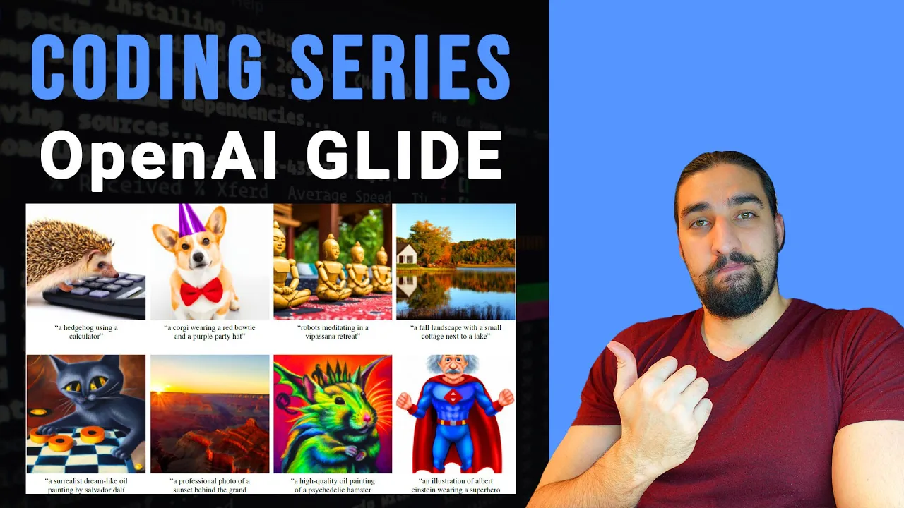

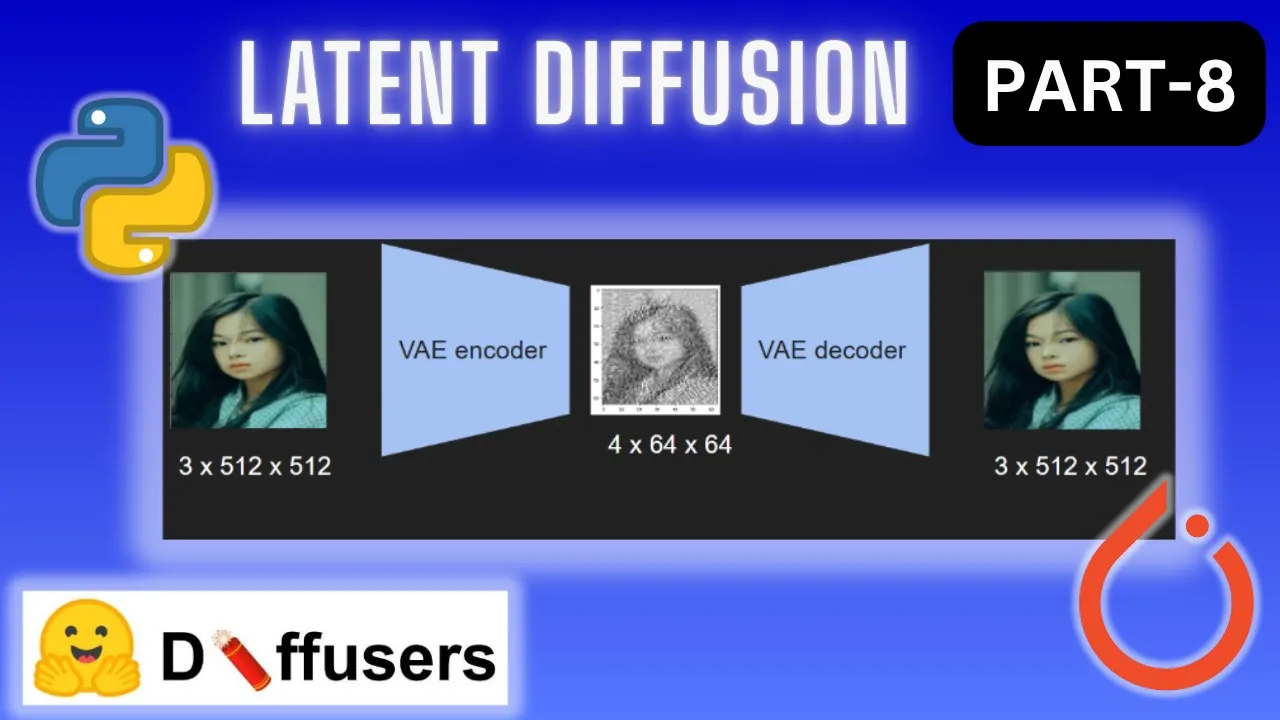


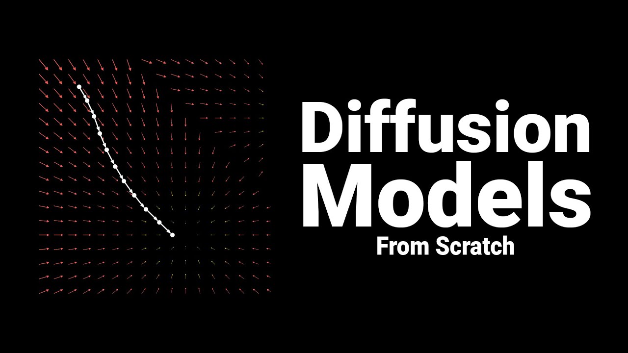


Denoising Diffusion Probabilistic Models (DDPM) are generative models that learn to reverse a gradual noising process, transforming random noise into meaningful data through a sequence of denoising steps; the implementation involves precomputing beta schedules for noise addition, training a neural network (such as a UNet) to predict noise at each time step, and sampling new data by iteratively denoising from pure noise using the learned model parameters.
Implementing Denoising Diffusion Probabilistic Models in PyTorch
Added:Proficiency in PyTorch, including building custom neural network architectures, managing training loops, and performing tensor manipulation.
Fundamental understanding of generative modeling concepts (e.g., latent variables, autoencoders, or GANs) and how they differ from discriminative tasks.
Basic probability theory and statistics, particularly Gaussian (normal) distributions, Markov chains, and noise addition processes.
Familiarity with the U-Net convolutional architecture, which serves as the standard backbone network for denoising in DDPMs.
Exploring Denoising Diffusion Implicit Models (DDIMs) to learn about accelerated, deterministic sampling techniques.
Implementing Classifier-Free Guidance (CFG) to transition from unconditional generation to conditional image synthesis (e.g., generating specific classes).
Studying Latent Diffusion Models (LDMs), such as Stable Diffusion, to understand how diffusion is scaled to high-resolution images by operating in a compressed latent space.
Investigating advanced mathematical formulations of diffusion, such as Score-Based Generative Models and Stochastic Differential Equations (SDEs).
3.7K views112likes10:19Original Release: 2024-06-15
welcome in that video we are going to implement the aome ddpm paper the noising different poting models uh yeah that's a really nice paper that had a major impact in the machine learning community on in generative AI in general uh that help the development of St of the division models and therefore that also an impact to the general public um so we're going to implement that paper we're going to uh implement it on the uh minist generation uh data task so these are results we get by the end of this video I will put the link of that of that GitHub in the in the description if you want to have a look at it uh if you use it and if it helpful to you please leave a thumbs up uh leave a stars but also yeah a thumbs up to the video um all that code is coming from my course on divion models so if you're interested at my course for now it's a best seller on UD um okay so let's have into the implementation we're going to spy torch to implement everything related to machine learning we're going to use scas but just foring the Min data we're not going to do any ml with scas on basically for the backbone so the function approximator in ddpm we're going to the unit that I implemented in in my latest YouTube videos so if you're interested into that you can have a look at it but D basically you can use any function approximator for the yeah for the function approximator you can use any uh any function with long parameters so you could use anything else at unit so basically you can really see this unit as a black box if you don't want to dive into it but if you want to understand how it's implemented or we use attention in it or we use the or we condition it based on the time stfy you can look at my latest videos um so yeah let's start by loading the data using caras we can also noriz the data so that there scale between zero and one and then we can also implement the helper to simple patch of data so we take his input bat size then we sample some poters in the training data and we uh we convert the the data those po into P torch transor we uh give them the proper size we used some in squeeing operation basically to put the the channel in the second dimension and then we push that to the device and lastly we interpolate the data to 32x 32 pixels because the unit wants input that have data multiple of of 16 and that's also the case in most division model implementation so for example if you have a look at stable division one or stable division two code you will see that when it's loading the data it is making sure that the data uh the size of the data the resolution is a multiple of 16 on if it's not it's scoping the data to to Ure that constraint uh so okay that being said we can directly move into implementing the divion model so we can take as input T the number of the total number of time set usually it's 1,000 the model that will be the function approximat in our case we're going to use a unit on the device that's going to be a usually Cuda we can uh create the uh the three main uh uh I'm not sure what to call those variables but beta alpha alpha bar are very common indion models if for the beta schedu we are going to use also something very common we're going to interpolate linearly between two values 1 E minus 4 on 0.02 and we're going to use the total number of time steps uh yeah um then we can move on to implementing the training function um again if you have more details about what are beta alpha alpha bar uh or or you to M more the training function you might want to have look at my course I did my best really make something very easy to understand on it's people really appreciate my course uh El are really focusing on the implementation so uh yeah if you're really interested to the implementation I think you're at the right place but if you have more a more technical understanding uh or or to have work through the paper my course is more adapted uh but B implementing the algorithm is very easy because it's just putting this P code into into code so yeah let's just do that let's put that into code so first we sample X from the training data and then we sample uniformly between one on Big T so let's just do that uh first we sample X from the training data then we sample T between zero on T um yeah here we need to be careful about the fact that uh yeah it's really you need to be careful about edges edges cases uh in in that implementation I I've decid yet to to to go from tal to one to t + one um that's really a choice as long as you're consistent everywhere in your code um yeah so once you've done that you sample Epsilon from normal distribution and then you take a gradiant step on that uh on that uh on that function uh on that's as easy as that so let's just Implement that uh that gradient step so we can because we have pre-computed Alpha bar for every time step T we can fetch it from our given type step T so here because I'm starting from one to t+ one I need to do this minus one again as long as you consistent that's fine so I'm Computing I'm predicting Epsilon with my function approximator in my case this a unit and then once I have all the variable I need to compute the equation we've just seen we can compute it and take the MC loss between the real exilon value and the predicted Epsilon value and then we can get take a Quant step on that on that loss so that's easy is that we're already done with the training function uh basically this training uh function is just doing one Grant step so we need to uh to call it multiple time in a training Loop we'll do that in a moment and then we can also Implement a function to S to sample from the division model and again this is just we just need to put this pseudo code into code so first we sample uh the U the noise from the normal distribution and then we will recursively uh or sequentially call the different model um so if T is greater than one we simple Z from the normal distribution otherwise we set to zero and then at every time step T we can Den noise XT using this equation so again very easy to put into code we first temple X randomly from normal distribution then uh we can iterate over the for T time step so yeah in our case 1,000 there subsequent paper that improve that for example if T is equal to 1,000 you need to do 1,000 step which is quite a lot on very slow on their papers that that allow to do that in 20 or 50 time steps using a better schedulers I will Implement that later so if you're interested subscribe um and there are also other papers that also try that will go to the extreme on push that to single step but this is with more Advanced Techniques such as dis I will also talk about that on that channel so again subscribe if you're interested so as we said we can sample Z from the normal distribution if this CR than one otherwise we set it to zero um and then yeah here I'm just doing some shaping here until now T is a single value but I want um I want T to have the same bch size as B I try to sample multiple data points in a single at the same time in parallel so I'm basically expanding the shape of T and then we can uh compute XT minus one from XT and for that we need beta T Alpha T Alpha bar T and therefore we can retrieve it from the because we've already PR computed them we can retrieve them for our time stfy and then we can compute basically what we are doing we simping XT minus one given from a normal distribution so what we do we compute the mean on the sigma the dev the standar deviation of the distribution so the summary statistics and then we can use them to compute x uh by sampling from this distribution and then yeah we can just add a three end one once we've done all our den noising steps we can return the latest value so we can return X on that's a simple as that now we can put put all the pieces together so we can um create our model we can create an Optimizer we can create a divion model by feeding the function approximator in our case that's a unit but again you can use any parametric model um and then we can train so basically it's uh it's super easy we just need to call this uh this training uh function this training step multiple times for a given number ofoc and then we can do a gradient step oh no sorry because we are already doing the gradient step in that training function so yeah we there is nothing else to do that's as simple as that we just need to call that function multiple times on that we can plot the results so we can sample a given number of images here we are going to sample 81 in parallel so that we can make a GD of 9 by9 images and then we can uh create the GD and plot the the images some one by one and then save the results and if you learn that code you should get results similar to what we've just seen before um yeah I really hope this code will be helpful to you if it is please leave a thumbs up it helps YouTube know this great content and subscribe for more content related to D model thank you
Up Next
29:29
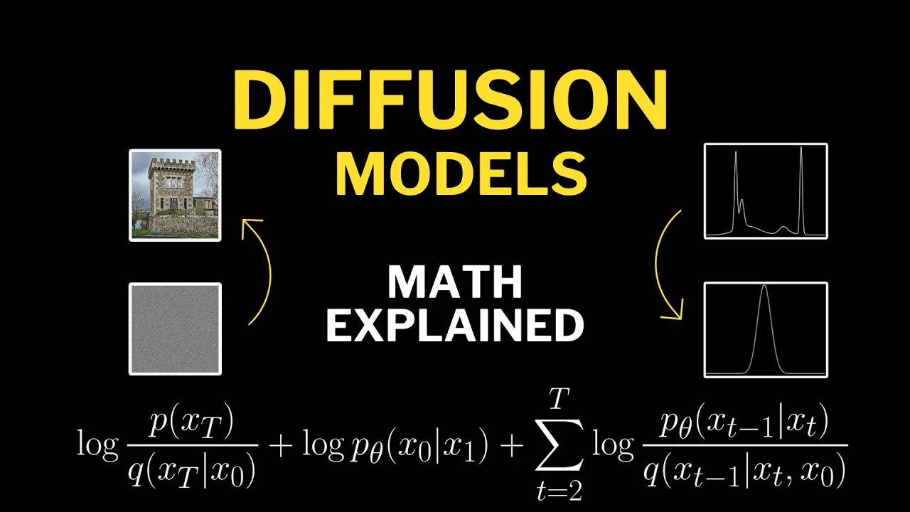
DDPM Explained: Denoising Diffusion Probabilistic Models
@Explaining-AI
98.8K views•2023-11-17

57:48
Secure Multiparty Computation (MPC): Foundations & Challenges
@SimonsInstitute
7.3K views•2015-05-28

13:03
Bypassing Tor Censorship: Bridges and Pluggable Transport Guide
@Coding_ForEveryone
397 views•2024-06-11

18:41
Neural Networks Explained: Math, Layers, and Learning Fundamentals
@3blue1brown
21.9M views•2017-10-05
Related Study Plans & Knowledge Roadmaps
Structured learning paths in Artificial Intelligence
artificial-intelligence
Aligning LLMs: DPO, TRL & Custom Datasets
01Foundations of Python & Machine Learning
02Transformers and Large Language Models (LLMs)
03Aligning LLMs: SFT and RLHF
+ 3 more learning modules
24h6 modules
Explore Roadmap
artificial-intelligence
Federated Learning: PyTorch, Flower & Privacy
01Python & Machine Learning Foundations
02Deep Learning Basics with PyTorch
03Introduction to Federated Learning
+ 2 more learning modules
35h5 modules
Explore Roadmap
artificial-intelligence
Securing LLMs: Guardrails AI & NeMo Gateway
01Introduction to LLMs, Python, and APIs
02Understanding LLM Vulnerabilities & Threats
03Defending LLMs with Guardrails AI
+ 2 more learning modules
15h5 modules
Explore Roadmap
artificial-intelligence
Building Recommenders: Two-Tower & Vector DBs
01Foundations of Python & Machine Learning Basics
02Introduction to Recommender Systems
03Deep Learning & Representation Learning
+ 3 more learning modules
75h6 modules
Explore Roadmap