Forward kinematics in RR robots uses trigonometric functions (sine and cosine) to calculate the end effector position by treating each joint as a right triangle, where the x-position is found by summing the cosine components of each limb (e.g., 1m × cos(30°) + 1m × cos(60°) = 1.366m) and the y-position by summing the sine components (e.g., 1m × sin(30°) + 1m × sin(60°)).
Forward Kinematics with Trigonometry | Robotics Basics
Added:Deep Dive
Basic Trigonometric Functions (understanding Sine, Cosine, and Tangent relationships in right-angle triangles).

What’s The ANGLE = ? Basic Trigonometry (sin, cos, tan)
13.3K
In a right triangle, the three basic trigonometric functions are defined as ratios of the sides. Sine (sin) is equal to the opposite side divided by the hypotenuse. Cosine (cos) is equal to the adjacent side divided by the hypotenuse. Tangent (tan) is equal to the opposite side divided by the adjacent side. These ratios are called trigonometric ratios because they represent comparisons between two values, essentially fractions that describe the relationships between the sides of a right triangle.
Click to watch →

SYNTube: FNDMATH LQ3 Part 1
273
The three basic trigonometric functions are sine, cosine, and tangent. In a right triangle with angle θ: sin(θ) = opposite/hypotenuse, cos(θ) = adjacent/hypotenuse, and tan(θ) = opposite/adjacent. Additionally, tan(θ) = sin(θ)/cos(θ).
Click to watch →

ixl alg1 HH.1 Trigonometric ratios sin cos and tan (v20.11a)
2.7K
In a right triangle, the three basic trigonometric functions are defined as follows: Sine (sin) of an angle equals the opposite side divided by the hypotenuse. Cosine (cos) of an angle equals the adjacent side divided by the hypotenuse. Tangent (tan) of an angle equals the opposite side divided by the adjacent side. These functions relate the angles of a right triangle to the ratios of its sides.
Click to watch →

Maths | How To | Sine (sin), Cosine (cos) and Tangent (tan)
138
Trigonometry uses six primary functions based on right-angled triangles. The three basic functions are sine (opposite/hypotenuse), cosine (adjacent/hypotenuse), and tangent (opposite/adjacent), remembered via SOHCAHTOA. The three reciprocal functions are secant (1/cos), cosecant (1/sin), and cotangent (1/tan). Key relationships include tan = sin/cos and the Pythagorean identity. These ratios remain constant for any given angle regardless of triangle size, enabling consistent calculations across different triangle dimensions.
Click to watch →

الدوال المثلثية ص99
110
In a right triangle, the three basic trigonometric functions are defined as ratios between sides: Sine (sin) = opposite/hypotenuse, Cosine (cos) = adjacent/hypotenuse, and Tangent (tan) = opposite/adjacent. For example, in a 3-4-5 right triangle, sin(θ) = 3/5, cos(θ) = 4/5, and tan(θ) = 3/4.
Click to watch →
Deep Dive
Cartesian Coordinate Systems (ability to plot points and understand X, Y axes in a 2D plane).

فيزياء الخامس العلمي | منهج 2025 | الفصل الاول | المحاضرة (1) 4K | أنظمة الاحداثيات
691.2K
The Cartesian coordinate system uses two perpendicular axes (x and y) to locate points in a plane. The x-axis is horizontal (positive right, negative left), and the y-axis is vertical (positive up, negative down). Points are represented as ordered pairs (x, y). To plot a point, start at the origin, move horizontally by the x-value, then vertically by the y-value. The plane is divided into four quadrants. This system is essential for describing positions in daily life, from restaurant ordering to military targeting.
Click to watch →
![[Full] Pembahasan Koordinat Kartesius](https://i.ytimg.com/vi/L9lGdwgamto/maxresdefault.jpg)
[Full] Pembahasan Koordinat Kartesius
12.9K
The Cartesian coordinate system consists of two perpendicular axes: the horizontal x-axis and vertical y-axis. Positive values extend right and up, while negative values extend left and down. To plot a point (x,y), move x units horizontally then y units vertically. The order is always x first, then y. Points on axes have one coordinate as zero. Negative coordinates indicate positions in opposite directions from the origin.
Click to watch →

PLANO CARTESIANO – COMO LOCALIZAR PONTOS E ENTENDER EIXOS X E Y
15.8K
The Cartesian plane consists of two perpendicular axes: the horizontal x-axis (abscissas) and the vertical y-axis (ordinates), intersecting at the origin (0,0). The plane is divided into four quadrants: Quadrant I (positive x, positive y), Quadrant II (negative x, positive y), Quadrant III (negative x, negative y), and Quadrant IV (positive x, negative y). Coordinates are represented as ordered pairs (x, y), where the first number indicates horizontal movement from the origin and the second indicates vertical movement. To locate a point, start at the origin, move horizontally by the x-value, then vertically by the y-value. Conversely, to find coordinates of a point, read its horizontal position on the x-axis and vertical position on the y-axis.
Click to watch →

الدرس 03: تعليم النقاط في المستوى ( المعلم المتعامد و المتجانس ) / الثانية متوسط (2م)
52.1K
A Cartesian coordinate system consists of two perpendicular (متعامد) and uniform (متجانس) axes: the horizontal axis (محور الفواصل) and the vertical axis (محور الترتيب), intersecting at the origin (المبدا). Points are located by their coordinates (x, y), where x represents the position on the horizontal axis and y represents the position on the vertical axis. To plot a point, draw perpendicular lines from the x and y values to their intersection. Points on the axes have one coordinate as zero: points on the horizontal axis have y=0, and points on the vertical axis have x=0.
Click to watch →

10 MENIT JAGO KOORDINAT KARTESIUS‼️LENGKAP
20.6K
The Cartesian coordinate system uses two perpendicular axes (x-axis horizontal, y-axis vertical) to locate points. Points are represented as ordered pairs (x, y), where x indicates horizontal position and y indicates vertical position. Positive x values are to the right, negative x values to the left; positive y values are above, negative y values below. To plot a point, start at the origin and move horizontally by the x-value, then vertically by the y-value. For example, point (9, -4) is 9 units right and 4 units down from the origin.
Click to watch →
Deep Dive
Fundamental Robotics Terminology (definitions of links, joints, degrees of freedom, and end-effectors).

Robotics and Automation (Lecture 1)
1.9K
Links are solid structural members of a robot, while joints are movable couplings between them. Degrees of freedom is the number of independent movements a robot can realize with respect to its base. For example, a joint allowing rotation about one axis gives one degree of freedom. These fundamental concepts are essential for understanding robot kinematics and motion planning.
Click to watch →
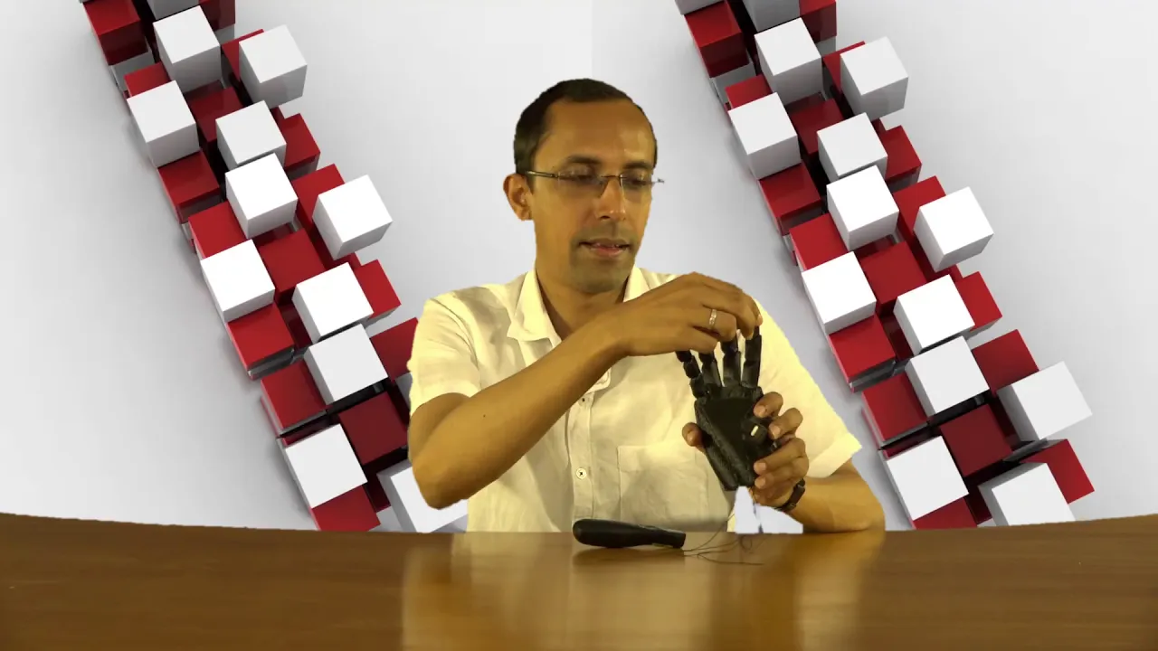
Introduction to Robotics | Dr. Nayan M. Kakoty | Tezpur University
541
Position represents translational location along X, Y, Z axes; orientation indicates rotational angles relative to these axes, together forming the pose. An end effector is the tool at a robot's end for tasks like gripping. Links are rigid connecting pieces between joints, while joints enable relative motion. Joint types include revolute (rotational), prismatic (linear), universal (two-axis rotation), and spherical (three-axis rotation). The work envelope defines the reachable volume for end effector operations.
Click to watch →

Lecture 2 | Introduction to Robotics
268.5K
A robot manipulator consists of links connected by joints, with the first link fixed as the base and the last link serving as the gripper. Two fundamental joint types exist: revolute joints enable rotation about a fixed axis, while prismatic joints enable translation along a fixed axis. Both provide exactly one degree of freedom. Generalized coordinates represent the minimal independent parameters needed to describe a robot's configuration. For a manipulator with n moving links and a fixed base, the degrees of freedom equal n because each joint imposes 5 constraints on the 6n initial parameters (3 for position, 3 for orientation per rigid body). This calculation assumes a fixed base; mobile robots like humanoids have additional base degrees of freedom.
Click to watch →

Lecture 01 Robotics: Primer-Robot Anatomy and Terminology
2.2K
Robotic systems are built from four fundamental components: joints, links, actuators, and sensors. Joints enable movement between links, with four primary types: revolute joints (1 DOF, rotational motion using θ), prismatic joints (1 DOF, linear motion using d), cylindrical joints (2 DOF, combination of prismatic and revolute), and spherical joints (3 DOF, representing roll, pitch, and yaw around x, y, z axes). Links connect joints and can be rigid or flexible. End effectors are specialized tools attached to robot wrists for performing tasks—grippers for grasping objects and tool grippers for processes like spray painting or spot welding. Different robotic applications use these components differently: humanoid robots use straight rigid links with electric actuators, exoskeletons employ series-connected mechanisms like four-bar linkages, and medical robots utilize prismatic joints for minimally invasive surgeries.
Click to watch →
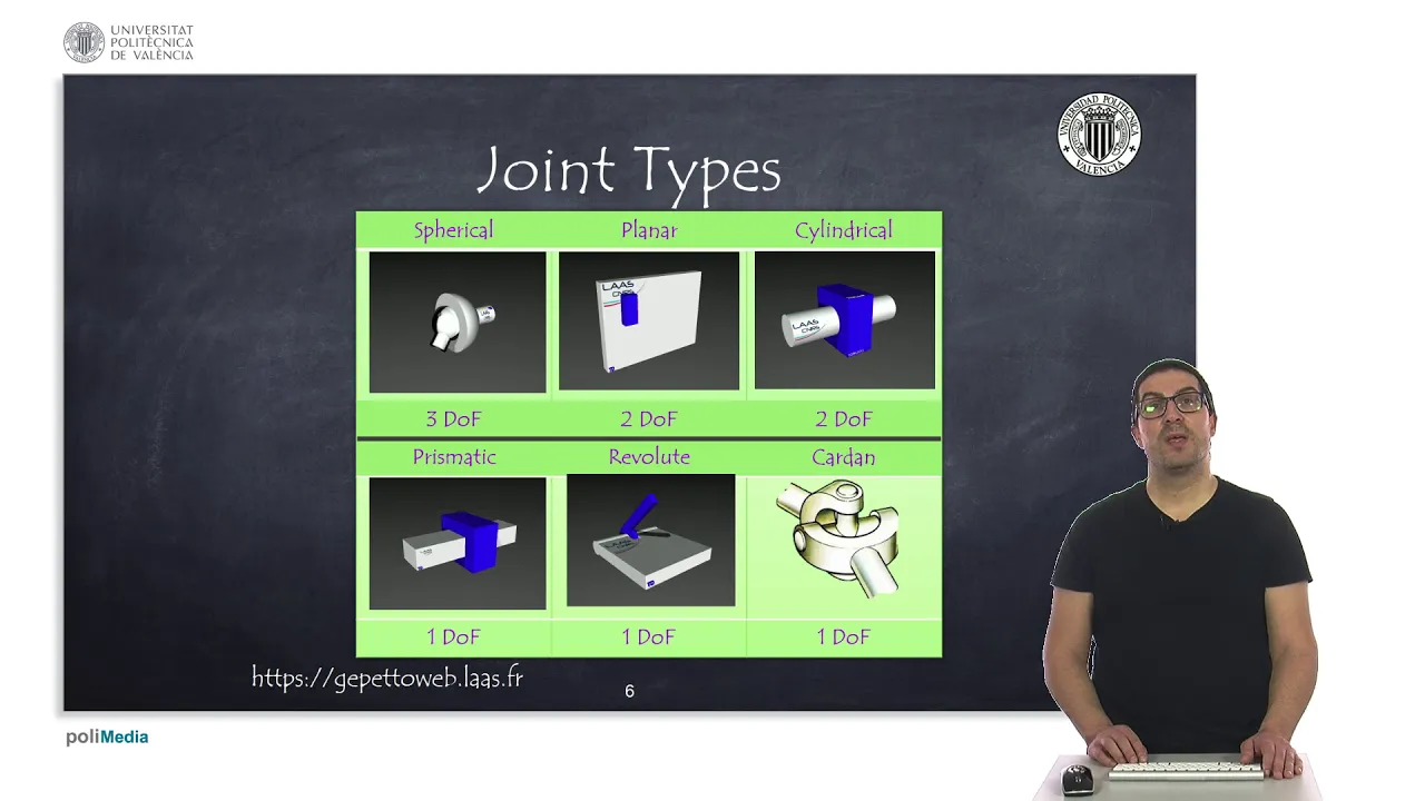
Robotic Systems: Joints, Links, and Degrees of Freedom Explained
4.8K
In robotic systems, a link is a movable rigid element with an associated reference frame, while a joint connects two links and constrains their movement in one or more directions (degrees of freedom); the mobility of an articulated system equals the number of independent moving elements (motors), and the two most common joint types are prismatic joints (which allow linear motion and are used in Cartesian robots with simple inverse kinematics but limited to 3 DOF) and revolute joints (which allow rotational motion and are more widely used in industrial applications due to being cheaper, lighter, and capable of controlling up to 6 DOF).
Click to watch →
Deep Dive
Basic Algebraic Manipulation (solving equations for unknown variables representing lengths and angles).

الدرس الثاني هندسة اولي اعدادي تابع العلاقات بين الزوايا
53.5K
When solving for an unknown angle represented by an algebraic expression, set up an equation using the appropriate geometric property. For example, if angles around a point are 2x - 1, 110, and 90 degrees, then (2x - 1) + 110 + 90 = 360. Solving: 2x + 199 = 360, so 2x = 161, and x = 80.5 degrees. When multiple angles around a point contain the same unknown variable, combine all terms and solve the equation.
Click to watch →

أهم 10 براهين في منهجك تالتة إعدادي ترم تاني 2026 📐 (مراجعة ليلة إمتحان الهندسة) 🔥
488
Algebraic equations can be solved by isolating the variable. For example, if 2s - 1 = s + 2, then s = 3.
Click to watch →

💥VCR? CONCURSO PM-PR l Relações Métricas no Triângulo Retângulo #2💥
2.8K
To find an unknown variable in an equation, isolate it using inverse operations. When x² is part of the equation, subtract known values from both sides to isolate x², then take the square root to find x. For example, if 8.41 = 4.41 + x², subtract 4.41 to get x² = 4, then x = √4 = 2. This algebraic process allows solving for unknown lengths in geometric problems by systematically applying mathematical operations.
Click to watch →

Homework 7-8 Geometry.
9.6K
When angles are given as algebraic expressions, set up equations to solve for unknown variables. For example, if 4x + 35 = 8x - 9, solve by subtracting 4x: 35 = 4x - 9, then add 9: 44 = 4x, so x = 11. Substitute x back into the angle expression to find the actual measure. Similarly, for 9x - 1 = 2x + 13, solve to find x = 2, then substitute to find the angle measure.
Click to watch →

ANGULOS... Cómo calcular el ángulo que falta, para alumnos de primaria.
16.1K
When an equation contains an unknown angle (represented by a variable like α), it is called an equation. To solve for the unknown, use the method of moving terms: if a term is being added on one side of the equality, it must be subtracted from the other side to maintain balance. For example, in the equation α + 55 = 180, to isolate α, subtract 55 from both sides: α = 180 - 55 = 125 degrees.
Click to watch →
Prerequisite Knowledge
- Concept 01Basic Trigonometric Functions (understanding Sine, Cosine, and Tangent relationships in right-angle triangles).
- Concept 02Cartesian Coordinate Systems (ability to plot points and understand X, Y axes in a 2D plane).
- Concept 03Fundamental Robotics Terminology (definitions of links, joints, degrees of freedom, and end-effectors).
- Concept 04Basic Algebraic Manipulation (solving equations for unknown variables representing lengths and angles).
Subsequent Learning
- Step 01Inverse Kinematics (calculating the required joint angles to place the end-effector at a specific target position).
- Step 02Homogeneous Transformation Matrices (using linear algebra and rotation matrices to represent position and orientation in 3D space).
- Step 03Denavit-Hartenberg (D-H) Parameters (a standardized convention for defining coordinate frames in multi-joint robotic arms).
- Step 04Jacobian Matrices and Differential Kinematics (calculating the velocity of the end-effector relative to joint velocities).
- Step 05Trajectory Planning and Control (programming smooth paths for the physical or simulated robot arm to follow).
RR Kinematics
RR Kinematics
0:00Playing Section
- 1
Uses trig to solve end effector position.
- 2
Sums angles and applies cosine, sine laws.
- 3
Results in 1.366m coordinate on plane.
Matrix-Based Methods and the Denavit-Hartenberg (D-H) Convention
While basic trigonometry (using right-angle triangles) is intuitive for simple 2D robotic arms, it becomes mathematically intractable and error-prone when applied to complex 3D systems with multiple degrees of freedom. To overcome these limitations, robotics engineers transition from manual geometric calculations to matrix-based methods, most notably the Denavit-Hartenberg (D-H) convention and Screw Theory (Product of Exponentials). These systematic approaches use linear algebra and homogeneous transformation matrices to model the position and orientation of each joint. By representing rotations and translations as standardized matrices, the forward kinematics of highly complex robots can be computed through sequential matrix multiplication. This matrix-centric paradigm is highly scalable, computationally efficient for computers to process, and serves as the industry standard for real-world robotic control and simulation, rendering manual trigonometric decomposition obsolete for anything beyond basic educational models.
Deep Dive
Inverse Kinematics (calculating the required joint angles to place the end-effector at a specific target position).

Forward and Inverse Kinematics (Classical & Neural Network Method)
4.3K
Inverse kinematics reverses the forward kinematics process: given a desired end effector position (X,Y), compute the required joint angles (θ1, θ2). For a 2-DOF arm, the analytical solution uses trigonometric identities and the law of cosines. First, compute D = √(X²+Y²) and verify it's within reach (D ≤ L1+L2). Then solve for θ2 using cos(θ2) = (X²+Y²-L1²-L2²)/(2L1L2), then find θ1 using θ1 = atan2(Y,X) - atan2(L2*sin(θ2), L1+L2*cos(θ2)). This allows robots to be commanded to specific positions rather than specific angles.
Click to watch →

Inverse kinematics. Explaining every step
50.3K
Inverse kinematics is a computational method that determines the joint angles required to position an articulated chain (such as a robotic arm or character limb) so that its end effector reaches a specified target location; the solution involves verifying reachability by comparing the target distance to the total arm length, then calculating angles using geometric principles like the law of cosines or circle intersections, with the iterative circle method being particularly effective for chains with multiple joints as it can be generalized to any number of segments by working backward from the target and using a pole vector to resolve ambiguous intersection choices.
Click to watch →

Cinemática Directa en Inversa de un Robot de 2 Grados de Libertad | Método Geométrico
33.4K
Inverse kinematics determines joint angles q1 and q2 given the end-effector position (x, y). First, compute the distance r = √(x² + y²) from origin to end-effector. Apply the law of cosines: cos(q2) = (l1² + l2² - r²)/(2*l1*l2). Use sin²(q2) + cos²(q2) = 1 to find sin(q2), yielding two solutions. The arctangent2 function determines q2 in all four quadrants. Then compute q1 by finding angle γ = arctan2(y, x) and angle β = arctan2(perpendicular distance, horizontal component), giving q1 = γ - β. Note that q1 depends on the previously computed q2.
Click to watch →

Inverse Kinematics of Robots | Robotics 101
138.7K
Inverse kinematics is the process of calculating robot joint parameters (such as link lengths and joint angles) to achieve a specified end-effector position and orientation, essentially working backward from the desired outcome rather than calculating the outcome from known joint angles as in forward kinematics; solving inverse kinematics involves setting up and solving systems of equations derived from forward kinematics, which can yield multiple mathematical solutions, though not all may be physically achievable in real-world applications.
Click to watch →
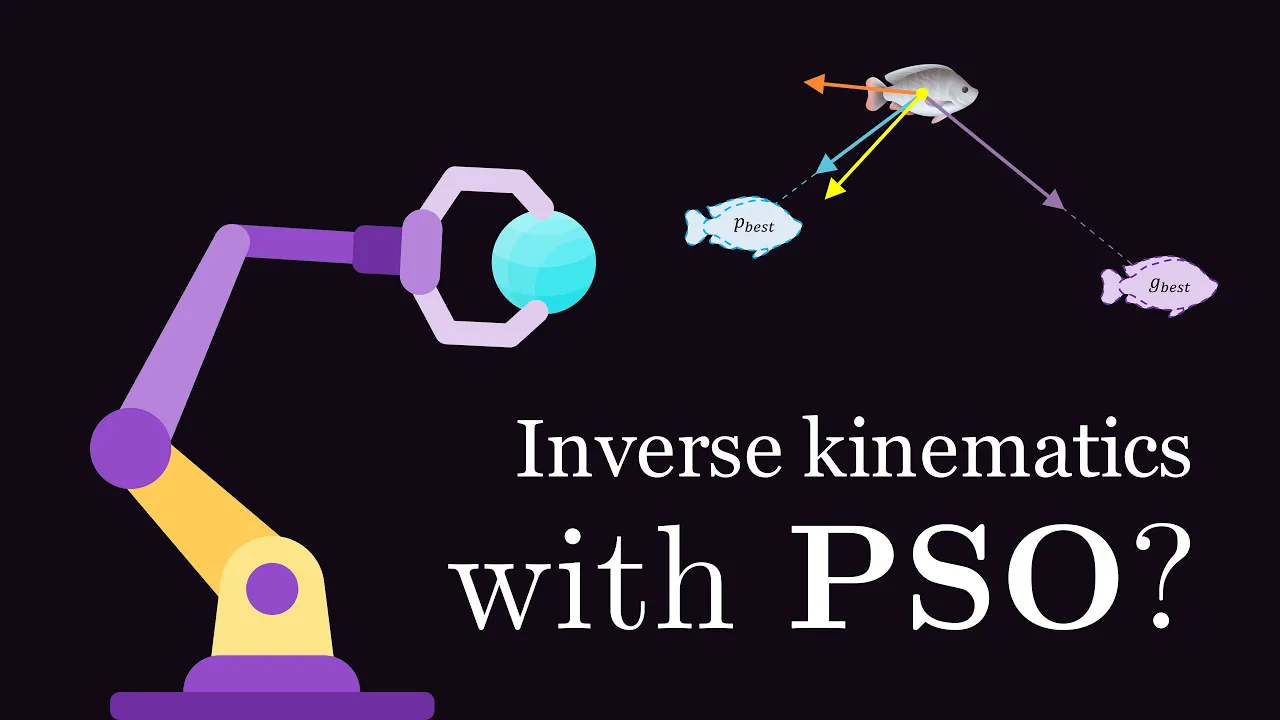
Controlling a robot arm with an unusual algorithm
48.1K
Robot arm control involves two fundamental mathematical processes: forward and inverse kinematics. Forward kinematics calculates the end-effector position given joint angles and segment lengths using trigonometry—each segment contributes x = l*cos(θ) and y = l*sin(θ), accumulating to find the final endpoint. Inverse kinematics reverses this process: given a target position (like catching a ball), find the joint angles that position the end-effector there. This forms an optimization problem minimizing Euclidean distance, constrained by fixed segment lengths and angular bounds of 0 to 2π.
Click to watch →
Deep Dive
Homogeneous Transformation Matrices (using linear algebra and rotation matrices to represent position and orientation in 3D space).

Modern Robotics, Chapter 3.3.1: Homogeneous Transformation Matrices
97.9K
Homogeneous transformation matrices are 4x4 matrices that combine position and orientation to represent rigid-body configurations. They consist of a 3x3 rotation matrix R and a 3x1 position vector p, with a bottom row of [0 0 0 1] for simplifying calculations. The set of all such matrices forms the special Euclidean group SE(3), which shares properties with rotation matrices: every matrix has an inverse, products yield valid transformations, and multiplication is associative but not commutative. Three primary applications exist: representing configurations, changing frame references using subscript cancellation rules, and displacing points or frames. Points require homogeneous coordinates (appending 1 to 3-vectors) for proper transformation. Any configuration results from first rotating then translating, making T both a configuration state and a transformation operator.
Click to watch →
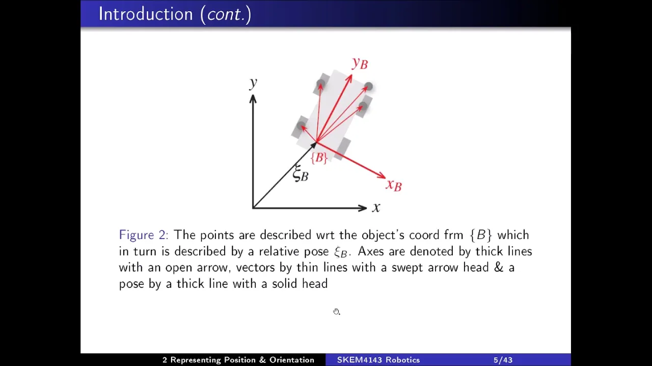
2 Representing Position & Orientation
2.8K
Three-dimensional homogeneous transformation matrices are 4×4 matrices combining 3×3 rotation matrices and 3×1 translation vectors. The matrix structure is [R, t; 0, 0, 0, 1], where R is the rotation matrix and t is the translation vector. Points are represented in homogeneous coordinates as 4×1 vectors with a 1 appended. Composition follows matrix multiplication: T^a_c = T^a_b × T^b_c, with rotation R^a_c = R^a_b × R^b_c and translation t^a_c = t^a_b + R^a_b × t^b_c.
Click to watch →

3D-gedruckter 6R-Roboter zum nachbauen! | Teil 2
51.1K
A homogeneous transformation matrix is a mathematical tool used to describe the pose (position and orientation) of a coordinate system. It consists of a rotation matrix and a position vector. The rotation matrix describes the orientation, with its first column representing the X-axis direction and the second column representing the Y-axis direction relative to the fixed coordinate system. The position vector gives the location of the origin of the body-fixed coordinate system relative to the fixed coordinate system. When a body rotates, the values in the rotation matrix change accordingly, allowing calculation of how the body's axes are oriented in space.
Click to watch →

4 Robot Arm Kinematics
15.6K
A homogeneous transformation matrix is a 4×4 matrix representing coordinate frame poses. It contains a 3×3 rotation submatrix (orientation) and a 3×1 position column (origin location), with the last row always [0 0 0 1]. Pure rotations about x, y, or z axes have specific matrix forms with cos(θ) and sin(θ) terms. Pure translations maintain identity rotation with only translation components changing. Position vectors must be expressed in homogeneous coordinates for proper transformation.
Click to watch →
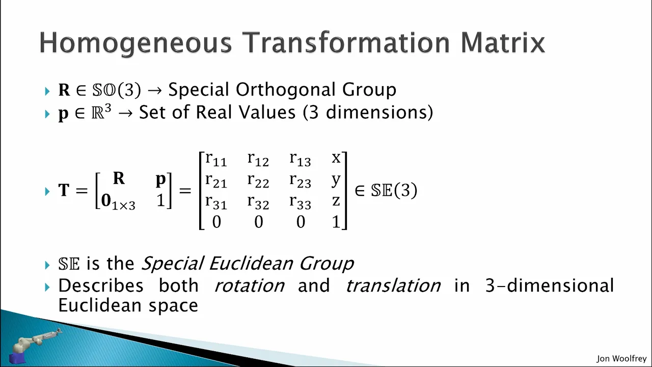
3.1 Transformation Matrices
17.5K
Homogeneous transformation matrices are 4x4 matrices that combine rotation and translation information for describing the relative position and orientation between reference frames. They consist of a 3x3 rotation matrix (from the Special Orthogonal group SO(3)) in the top-left corner, a 3x1 translation vector in the top-right, and a bottom row of [0 0 0 1]. This format enables mathematical operations to combine rotations and translations, which cannot be directly concatenated as a 3x4 matrix. These matrices belong to the Special Euclidean group SE(3) and describe both rotation and translation in three-dimensional Euclidean space.
Click to watch →
Deep Dive
Denavit-Hartenberg (D-H) Parameters (a standardized convention for defining coordinate frames in multi-joint robotic arms).

Denavit - Hartenberg (DH) Tables For Robotic Systems - Direct Kinematics II
231.9K
The Denavit-Hartenberg (DH) representation is a systematic method for describing the position and orientation of robotic joints using four parameters: a_i-1 (link length, distance between joint axes along the common perpendicular), alpha_i-1 (link twist, angle between joint axes about the common perpendicular), d_i (link offset, distance between origins along the previous joint axis), and theta_i (joint angle, rotation about the current joint axis). For prismatic joints, d_i is non-zero while theta_i is zero; for revolute joints, theta_i is non-zero while d_i is zero. These four parameters are organized into a DH table, which enables the calculation of transformation matrices that describe the spatial relationship between consecutive frames in a robotic manipulator.
Click to watch →
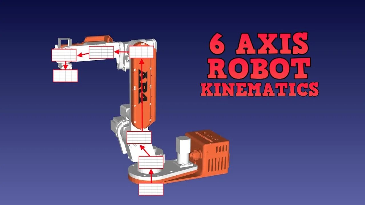
6 Axis Robot Forward & Inverse Kinematics Tutorial - Denavit Hartenberg Parameters With the AR4-MK2
59.9K
DH parameters are a shortcut method created in 1955 by Denavit and Hartenberg to create transformation matrices more easily using only four parameters per joint instead of six. The four parameters are: θ (theta) - joint angle about previous Z-axis; α (alpha) - angle about common normal from old Z to new Z; d - offset along previous Z to common normal; a - length of common normal. Four rules must be followed: Z-axis must be the rotation axis, X-axis must be perpendicular to both Z-axes, Y-axis follows the right-hand rule, and X-axis must intersect the previous Z-axis.
Click to watch →

Cinemática Directa: Parámetros de Denavit Hartenberg
98.7K
The Denavit-Hartenberg (D-H) convention provides a systematic method for representing robot kinematics using four parameters per joint: link length (a), link twist (alpha), link offset (d), and joint variable (theta or d). The procedure involves: (1) establishing a functional representation of the robot at its home position, (2) assigning coordinate frames following specific rules (z-axes along joint axes, x-axes perpendicular to adjacent z-axes), (3) filling the D-H parameter table with constant and variable parameters, (4) constructing homogeneous transformation matrices for each joint, and (5) multiplying these matrices to obtain the overall transformation from base to end-effector. This method enables precise mathematical modeling of robot kinematics for both planar and spatial manipulators.
Click to watch →
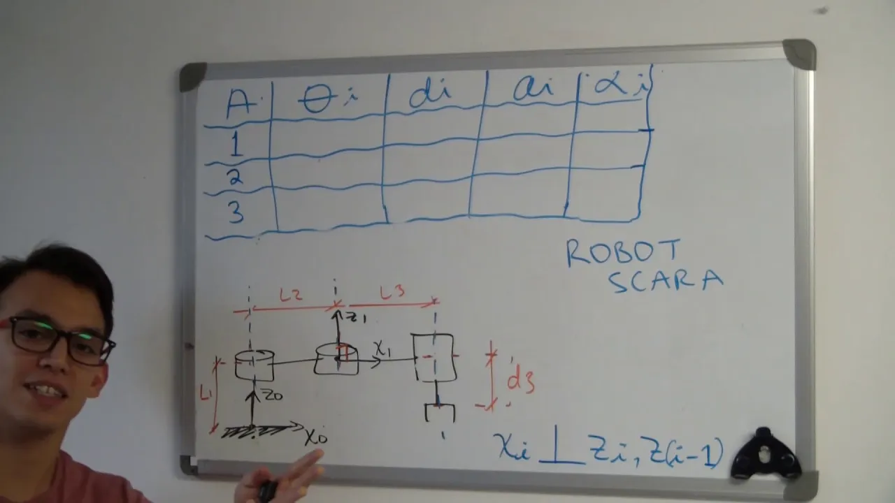
INTRO A CINEMÁTICA DE MANIPULADORES Y ROBOT SCARA
9.3K
The four DH parameters define the relationship between consecutive coordinate frames: Theta (θ) is the rotation angle about the z-axis to align x-axes; D (d) is the distance along the z-axis between origins; A (a) is the distance along the x-axis between origins; Alpha (α) is the rotation angle about the x-axis to align z-axes. For prismatic joints, the rotation angle θ is zero since no rotation occurs.
Click to watch →

Aula 5: Notação de Denavit-Hartenberg
13.1K
The Denavit-Hartenberg (DH) parameters are four parameters (theta, d, a, alpha) used to standardize coordinate systems for robot kinematic chains. Developed in 1955 by Denavit and Hartenberg, this convention remains widely used in robotics for solving manipulator kinematics. A robot manipulator consists of n rigid links connected by joints forming a kinematic chain. Links are numbered from 0 (base) to M (end effector). Each link has two parameters: 'a' (link length along X-axis) and 'alpha' (twist angle between Z-axes). Each joint has two parameters: 'd' (offset along Z-axis) and 'theta' (rotation angle about X-axis). For rotational joints, theta is variable; for prismatic joints, d is variable. The DH method uses homogeneous transformation matrices (4x4) to represent movements between joints. The DH method requires fixing a local coordinate frame on each link. The Z-axis of each frame aligns with the joint axis connecting to the next link, following the right-hand rule based on joint rotation direction. The origin is placed at the intersection of the current Z-axis and previous X-axis. If Z-axes intersect, origin is at intersection; if parallel, origin is at joint articulation. The X-axis must be perpendicular to both current and previous Z-axes. The Y-axis is determined by the right-hand rule.
Click to watch →
Deep Dive
Jacobian Matrices and Differential Kinematics (calculating the velocity of the end-effector relative to joint velocities).
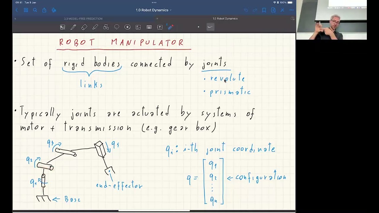
Lecture 2 - Optimization and Learning for Robot Control - Robot kinematics and dynamics
411
Differential kinematics computes the end-effector's linear and angular velocities from joint velocities. For revolute joints, velocity is calculated as the cross product of the rotation axis and lever arm vector, scaled by joint velocity. This relationship shows that end-effector velocity is a linear function of joint velocities. The Jacobian matrix J combines these contributions into a 6×n matrix mapping joint velocities to 6D end-effector velocities (V = J × Q dot). The Jacobian has a dual role: mapping velocities forward and torques backward through τ = J^T × W, enabling prediction of how robot motion affects tool tip behavior and how external loads translate to joint torques.
Click to watch →
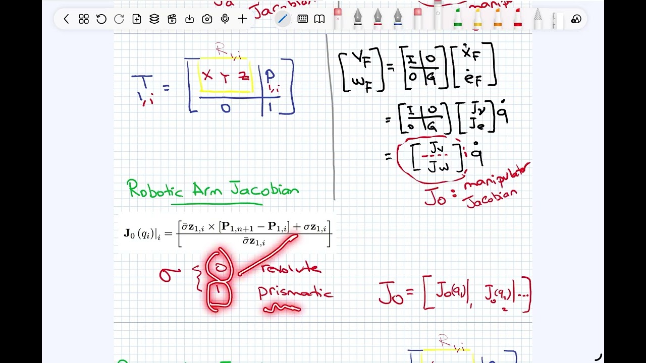
Jacobin Matrix, Robots velocity kinematics
243
The Jacobian matrix is a fundamental mathematical tool in robot kinematics that transforms joint velocities (q_dot) into end-effector linear velocity (v) and angular velocity (ω) through the relationship v = J × q_dot and ω = J_angular × q_dot, where J is the Jacobian matrix and J_angular is the angular velocity matrix; for a robot with n joints, the Jacobian matrix has n columns, with each column representing the partial derivative of the end-effector position with respect to each joint variable, enabling the calculation of end-effector motion from joint space velocities.
Click to watch →
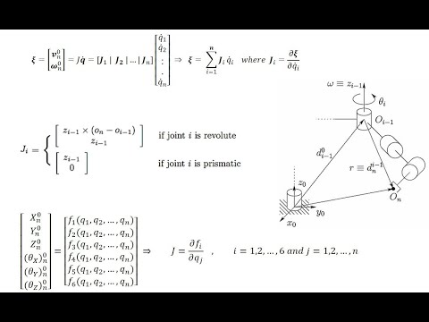
Differential Forward Kinematics Part 2: Manipulator Jacobian, Analytical vs Geometric Jacobian
6K
The Jacobian can be calculated using partial derivatives of the forward kinematics equations. If the end effector position (x, y, z) and orientation angles (θx, θy, θz) are expressed as functions of the joint variables (q1 to qn), then taking the time derivative using the chain rule gives: ζ = [∂(f1)/∂q1 ∂(f1)/∂q2 ... ∂(f1)/∂qn; ∂(f2)/∂q1 ∂(f2)/∂q2 ... ∂(f2)/∂qn; ...; ∂(f6)/∂q1 ∂(f6)/∂q2 ... ∂(f6)/∂qn] × q̇. For a three-degree-of-freedom planar arm, this yields: J = [[-a1sin(θ1) -a2sin(θ1+θ2) -a3sin(θ1+θ2+θ3); -a2sin(θ1+θ2) -a3sin(θ1+θ2+θ3); -a3sin(θ1+θ2+θ3)], [a1cos(θ1) + a2cos(θ1+θ2) + a3cos(θ1+θ2+θ3); a2cos(θ1+θ2) + a3cos(θ1+θ2+θ3); a3cos(θ1+θ2+θ3)], [1 1 1]]. Each element ∂(fi)/∂qj represents how much the ith component of end effector velocity changes per unit change in the jth joint velocity.
Click to watch →

Modelo Diferencial (Velocidades) - Jacobiana Directa - Robótica
893
To compute end-effector velocities for a specific robot configuration, the Jacobian matrix is multiplied by the vector of joint velocities. For example, with q̇₁ = π/2 rad/s, q̇₂ = π/2 rad/s, and q̇₃ = 1 m/s, the end-effector velocities are obtained by J × [q̇₁, q̇₂, q̇₃]ᵀ. The result is a 6×1 vector containing the three linear velocity components (vₓ, vᵧ, v_z) and three angular velocity components (ωₓ, ωᵧ, ω_z). This calculation enables real-time prediction of end-effector motion for any given joint velocity configuration, demonstrating practical application of the Jacobian in robot control.
Click to watch →

How to find Jacobian Matrix? | Solved Examples | Robotics 101
31.4K
The Jacobian matrix maps joint velocities to end-effector velocities through the relationship x_dot = J * θ_dot, where x_dot represents the combined linear and angular velocity of the end-effector, and θ_dot represents the joint velocities; to compute the Jacobian, first perform forward kinematics to derive the displacement vector d and orientation angle φ as functions of joint angles, then differentiate these with respect to time to obtain the linear and angular velocities, and finally express the velocity vector as a linear combination of the joint velocity terms to populate the Jacobian matrix.
Click to watch →
Deep Dive
Trajectory Planning and Control (programming smooth paths for the physical or simulated robot arm to follow).

Un petit tour sur les bras robot multi axes.
270
Robot arms use trajectory planning to move between positions smoothly. Methods include constant acceleration/deceleration phases or breaking movements into multiple steps. Control functions take target angles for all axes and move the arm to those positions. The program continuously monitors current positions and adjusts motor outputs. This allows the arm to move to any position within its range of motion while maintaining smooth, controlled movement throughout the trajectory.
Click to watch →
Robotics 1 - Introduction, part 1 (Lecture 1)
3.3K
A trajectory consists of a geometric path (sequence of points parameterized without time) and a timing law (assigning time to each point). This separation allows programming paths slowly and executing at fast speeds by scaling timing. Trajectories can be planned in joint space or Cartesian space. Control systems integrate sensors, actuators, and commands through local control loops at each joint that receive velocity references and apply appropriate torques. The course assumes local controllers can accurately follow velocity references, treating the robot as a kinematic system initially before advancing to dynamics.
Click to watch →

Trajectory Planning
254
Trajectory planning is the process of determining smooth time functions that describe robot motion from initial to final positions. It involves two coordinate spaces: joint space (using joint angles, velocities, accelerations) and Cartesian space (using position and orientation). Joint space planning offers advantages in motion control and collision detection, while Cartesian space planning requires inverse kinematics and faces singularity challenges. The planning process involves task sequence determination, point interpolation, and inverse kinematics application to generate smooth motion paths.
Click to watch →

Trajectory Planning and Generation | Cubic Polynomials | Parabolic Blends | Robotics
61.7K
Trajectory planning involves generating the time history of position, velocity, and acceleration for robotic manipulators. Users specify desired positions and orientations without computing complex equations. Trajectories are computed at runtime with path update rates of 60-2000 Hz. Smooth motion is essential to prevent vibrations and reduce wear on robot links. Waypoints (wire points) ensure smooth paths by imposing constraints. Two main methodologies exist: joint space schemes using joint angles (easier to compute) and Cartesian schemes using frame positions/orientations (higher computational burden).
Click to watch →
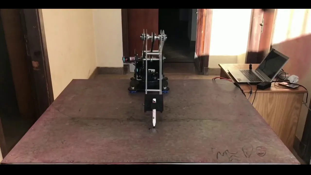
Trajectory planning for Four degrees of Freedom Robot Arm Using MATLAB
247
Trajectory planning for a four degrees of freedom robot arm involves generating motion paths in Cartesian space using MATLAB's robotics toolbox, with trajectory timing laws and PID control for precise motion execution, while the system model and simulation are conducted using Simulink.
Click to watch →
RR Kinematics
RR Kinematics
0:00- 1
Uses trig to solve end effector position.
- 2
Sums angles and applies cosine, sine laws.
- 3
Results in 1.366m coordinate on plane.
Matrix-Based Methods and the Denavit-Hartenberg (D-H) Convention
While basic trigonometry (using right-angle triangles) is intuitive for simple 2D robotic arms, it becomes mathematically intractable and error-prone when applied to complex 3D systems with multiple degrees of freedom. To overcome these limitations, robotics engineers transition from manual geometric calculations to matrix-based methods, most notably the Denavit-Hartenberg (D-H) convention and Screw Theory (Product of Exponentials). These systematic approaches use linear algebra and homogeneous transformation matrices to model the position and orientation of each joint. By representing rotations and translations as standardized matrices, the forward kinematics of highly complex robots can be computed through sequential matrix multiplication. This matrix-centric paradigm is highly scalable, computationally efficient for computers to process, and serves as the industry standard for real-world robotic control and simulation, rendering manual trigonometric decomposition obsolete for anything beyond basic educational models.
Basic Trigonometric Functions (understanding Sine, Cosine, and Tangent relationships in right-angle triangles).
Cartesian Coordinate Systems (ability to plot points and understand X, Y axes in a 2D plane).
Fundamental Robotics Terminology (definitions of links, joints, degrees of freedom, and end-effectors).
Basic Algebraic Manipulation (solving equations for unknown variables representing lengths and angles).
Inverse Kinematics (calculating the required joint angles to place the end-effector at a specific target position).
Homogeneous Transformation Matrices (using linear algebra and rotation matrices to represent position and orientation in 3D space).
Denavit-Hartenberg (D-H) Parameters (a standardized convention for defining coordinate frames in multi-joint robotic arms).
Jacobian Matrices and Differential Kinematics (calculating the velocity of the end-effector relative to joint velocities).
Trajectory Planning and Control (programming smooth paths for the physical or simulated robot arm to follow).
154 views0likes3:00@HansolarEngineeringOriginal Release: 2025-10-17
you the joints of an RR robot are angled at 30° and 30° for example. Let's go and take a look at forward kinematics of that. All right, so you have your robot's base and I tell you from the ground it lifts up by 30° and then I tell you the second joint lifts up by 30°.
Where is your endeector? Now people, this is basic trigonometry.
What I mean by basic trigonometry is this is a right angle triangle. This is also a right angle triangle the 30° and you add it to the 30°. This is essentially a right angle triangle at 60°. So let's go and find out where our xaxis is. And how do we do that? Okay, so we have to work it out for this one and this limb. All right, and this so basically after the first 30° we'll be able to find exactly where this midpoint is. And then when we add it to the second limb position that we're going to use the trigonometry for uh you'll find your exact x position. Now let's go and look at how to do it. All right. So you'll take the 1 m limb length and multiply it by cos 30. And then it's obviously your first limb. Then what you go and do is you take the 1 m limb length of the second one and then multiply it by cos 60. Why cos 60?
Because you take this, you take this angle and you add it to that angle.
1.366 m is your x position. It'll be 1 m * sin 30 + 1 m * sin 60. All right. And it gives you the exact same 1.366 m. All right. So your your effective position on a your effective position on a cartisian plane this is 2 m it's 1.366 and over here it would be the same thing 1 m 2 m so it'll be around there's your position I know it's a very basic descriptive position but you understand how forward kinematics work you the joints of an RR robot are angled at 30° and 30° for example let's go and take a look at forward kinematics of All right. So, you have your robot's base and I tell you from the ground it lifts up by 30° and then I tell you the second joint lifts up by 30°.
Where is your endector? Now people, this is basic trigonometry. What I mean by basic trigonometry is this is a right angle triangle. This is also a right angle triangle. The 30° and you add it to the 30°. This is essentially a right angle triangle at 60°. So let's go and find out where our xaxis is. And how do we do that? Okay, so we have to work it out for this one and this limb. All right, and this so basically after the first 30°, we'll be able to find exactly where this midpoint is. And then when we add it to the second limb position that we're going to use trigonometry for, uh, you'll find your exact X position.
Up Next
68:11
Introduction to Robotics: Kinematics & Manipulator Fundamentals
@stanford
268.5K views•2008-07-22

58:25
MathWorks Virtual RoboSub Simulation Environment | Webinar 2026
@RoboNationInc
209 views•2026-03-10

11:04
How to Build a Self-Balancing Robot: Arduino Nano & MPU6050
@easytechzones
16.8K views•2022-03-09

25:22
Micromouse: The Fastest Maze-Solving Robots on Earth
@veritasium
23.5M views•2023-05-24
Related Study Plans & Knowledge Roadmaps
Structured learning paths in Robotics
robotics
Building Delta Robots: Kinematics & Pico
01Foundations of Delta Robots & Mechanical Design
02Electronics and Microcontroller Setup with Pi Pico
03Delta Robot Kinematics and Coordinate Math
+ 3 more learning modules
65h6 modules
Explore Roadmap
robotics
Building Ballbots: Dynamics, Kalman & LQR
01Embedded Electronics & Omniwheel Actuation
02Ballbot Kinematics & Rigid Body Dynamics
03IMU Sensors & Kalman Filter State Estimation
+ 2 more learning modules
42h5 modules
Explore Roadmap
robotics
Micromouse: Hardware, PID Control & Flood-Fill
01Electronics & Teensy Microcontroller Basics
02Sensors and Actuators: Motors, Encoders & IR
03Precision Movement: Implementing PID Control
+ 2 more learning modules
35h5 modules
Explore Roadmap
robotics
CDPR: Kinematics, Arduino & Winch Control
01Foundations of Arduino & Basic Electronics
02Stepper Motors and Winch Mechanics
03Kinematics of 2D Cable-Driven Robots
+ 2 more learning modules
28h5 modules
Explore Roadmap