Ozone Monitoring From Space: TEMPO Satellite & Air Quality Webinar

[00:00:00]All right, as a reminder, we are recording today. So, if you don't want to be on the recording, uh feel free to turn off your camera. Um we will be posting this on our YouTube channel for viewing later for those who can't make it. Uh so, welcome to our second installment for the Ozone Garden Network uh summer webinar series. We're excited to have you here with us. Um we're excited to have a special guest presenting with us today. Uh so, today we have Dr. Hi Sunung Chong who's a physicist in the atomic and molecular physics division at the center for astrophysics Harvard and Smithsonian.

[00:00:34]His interests lie in retrieval of ga trace gas concentrations and earth's atmosphere from remote sensing instrument instruments and calibration of remote sensing instruments as well.

[00:00:46]Um he is a investigator on NASA's measures project to build long-term satellite data records for trace gas concentrations and our very own tempo instrument as well. And we're excited to have him here with us today uh to talk a little bit about uh measuring monitoring ozone from the ground and space. Thank you so much for being here with us doc uh Dr. Chong. I'll let you take it away.

[00:01:13]>> Thank you very much. Uh let me share my screen.

[00:01:24]Yeah. So thank you Erica for the uh very nice introduction and I thank Emma and the Ozone Garden group for having me here. Um my name is Hang Chong and I'm from Center for Astrophysics Harvard and Smithsonian and it's an honor to be presenting this webinar um as someone who produces satellite data. It's always a pleasure to connect with potential users and discuss possible applications.

[00:01:50]So, uh today I'll be um talking about monitoring ozone from the ground and space.

[00:01:59]Um so this is the outline of my presentation today. uh first I will be describing how ozone functions as a pollutant in the atmosphere and then I will be talking about ground level or surface ozone measurements over North America. Then I'll move on to satellite remote sensing and then specifically uh I'll be talking about tempo tropospheric emissions monitoring of pollution uh which is the satellite mission I've been working on. Um so uh the air pollution as you know is not just a recent issue. So some studies found that atmospheric lead pollution over Europe during the Roman era was already significant. So uh it it has been significant for a long time. Um but the regulation of urban smoke began mainly in the 1940s uh following severe pollution events. So that's why I I brought some examples of air pollution from 1940s and 50s here.

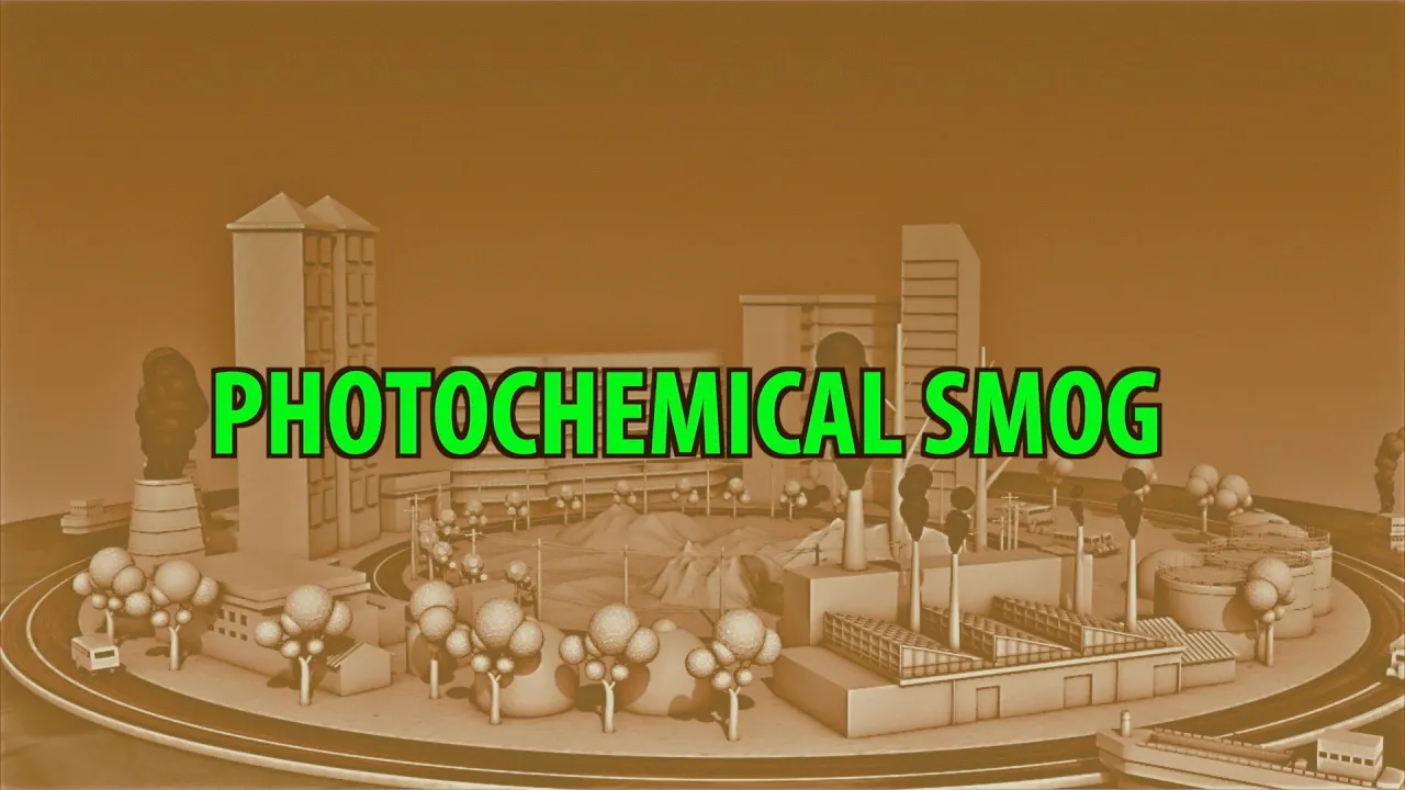
[00:03:09]So in 1940s um smoke was severe in Los Angeles and then in 1947 um Los Angeles air pollutant uh air pollution control district forms and in 1948 Donora Pennsylvania had a smoke disaster and in 1949 uh national symposium uh there was national symposium on air pollution in Los Angeles and in 1951 uh Oregon approves agency to control air pollution and 1952 air pollution disaster in London and then mid 1950s ozone levels in Los Angeles uh reach 65 ppm and for context the current air quality standard for ozone is 007 ppm so this is really high and in 1955 Eisenhower asks Congress to examine air pollution. So the key word here in this slide is smoke. So uh the smoke is a blend word formed from smoke and fog and there are two major types of smoke. Um here the first one is London smoke and it is also called classical smoke and typically the color of the sky when this smoke is present is gray and then typically we find this smoke in winter and that's because the weather condition should be involving low temperature and stagnant air and the major sources uh of this smoke include cold burning and the key Components of this smoke include surfer dioxide and surfate aerosols. On the other hand, Los Angeles smoke has different characteristics. So this is also called photochemical smoke and then the typical color of this smoke is brown and usually we find this smoke in summer and that's because the weather condition should be involving high temperature and intense sunlight.

[00:05:24]uh and the major source is also different from uh the London smoke. So the major source from for Los Angeles smoke is high vehicle traffic usually and then the key components involve nitrogen oxide which we call NOX or NOx uh volatile organic compounds VOCC's and ozone.

[00:05:48]Um from 1995 to 2023 uh there was a 96% reduction in sulfur dioxide emissions from power plants. So this is a huge reduction uh 96% and it's mainly through policies such as clean air act and acid rain program. Um so in this presentation I'll be discussing air pollution similar to the Los Angeles smoke. Um so today's uh pollutant of interest uh is of course ozone. Uh but NOx and VOCC's will also be mentioned as they are key precursors to ozone formation. Uh and similar to sulfur dioxide nitrogen oxide emissions have also been decreased significantly and the impact will be discussed uh later in this presentation.

[00:06:45]uh as a simplified example um I I brought this uh primary uh primary colors of light to describe why Los Angeles smoke is brownish. Um so as a simplified example imagine we lose blue from these three primary colors of light and then what remains is yellow and of course uh this reality is a bit more complex than that. Uh so nitrogen dioxide absorbs uh blue light and light contains a full spectrum of colors not just uh these three. Um so this is the actual color of nitrogen dioxide. So here in this lab concentrated nitric acid reacting with copper and generating nitrogen dioxide gas. And as you can see this this color is close to brown uh or reddish. Uh so this example uh provides us a hint at the basic principle behind satellite observation. Basically we examine what color is missing in the light observed by the satellite. But instead of using this several colors we use hundreds or thousands of wavelength.

[00:08:03]uh and instead of using only visible wavelength, we also utilize ultraviolet and near infrared uh wavelengths. So that's how we use satellite to observe air pollutants.

[00:08:18]And uh today's pollutant of interest ozone is present throughout different layers of the earth's atmosphere. And in our field, the EPA and other scientists uh tend to say there are good ozone and bad ozone. However, it's not that they are chemically different. They are exactly the same molecule. But depending on where they are located, their role changes from our perspective. Uh first in the stratosphere, the ozone layer protects us from uh UV. Uh so it functions as UV shield in the stratosphere. Uh but in the troposphere below 8 or 10 kilometers altitude uh in the upper troposphere ozone functions as a greenhouse gas. So tropospheric ozone uh is not only air pollutant but also greenhouse gas. And in the middle troposphere ozone is a source of um hydroxil radical. And we we call this ozone background ozone. And then in the boundary layer, ozone functions as a pollutant. And that's because we breathe in the boundary layer.

[00:09:36]So the ground level or bad ozone uh is not emitted directly into the air. First here nitrogen oxide or NOx and volatile organic compounds or VOCC's are emitted into the atmosphere.

[00:09:53]Uh major sources of NOx and VOCC's include um industrial facilities, electric utilities, motor vehicle exhaust, gasoline vapors uh and chemical solvents. So then chemical reactions between KNOPS and VOCC's create ozone in the presence of heat and sunlight.

[00:10:20]So we refer to ground level ozone as bad ozone. But in what sense is it bad? Uh first ozone pollution has health effects. Depending on the level of exposure, ozone can cause coughing and sore or scratchy throat and ozone can make it more difficult to breathe deeply um and can cause pain when taking a deep breath. So uh there are uh many more health effects of ozone pollution. So that that's why we call uh ground level ozone as bad ozone. Um and also second ozone pollution has ecosystem effects.

[00:11:02]The uh this aspect uh this aspect is highly related to the ozone garden activities. So when sufficient ozone enters the leaves of a sensitive plant, it can reduce photosynthesis and it can slow the plant's growth and it can increase sensitivity sensitive plants risk of disease, damage from insects, effects of other pollutants and harm from severe weather.

[00:11:30]Um so that that's the effects of ozone pollution on health and ecosystem.

[00:11:36]So before we focus on the uh United States, I'd like to present this global view of ozone pollution. So on the left I'm presenting um global non-urban daytime average surface ozone from 2000 to 2014.

[00:11:56]And this season is summer uh June, July, August. And on the right I'm presenting the same quantity but for winter, December, January and February. So during the summer uh the first thing we can notice is that the concentrations of ozone are higher than in winter.

[00:12:16]And uh that's because uh as I uh mentioned in the previous slides the ozone production involves sunlight and heat and the emissions of precursors including NOx and VOCC's. So the high concentrations of ozone are found urban areas where we we have more emissions of those precursors. Uh so we have uh Los Angeles here. um as we u briefly cover in the previous slide and also uh southern Europe has high ozone concentrations and also in Asia we can also observe high ozone concentrations.

[00:12:58]On the other hand, in the winter season, uh the high concentrations of ozone are not necessarily related to uh the emissions of NOx and VOCC's or sunlight.

[00:13:11]Uh because an altitude or elevation of the terrain also plays some role here.

[00:13:17]So that's why we see this high concentration of ozone here. Uh and that's because ozone is uh present throughout the different levels of atmosphere. um as described in the previous slide.

[00:13:30]Uh so here we we can uh see that uh in the summer season ozone concentrations are uh typically higher. So this season is also called ozone season. Um and uh now now let's focus on the United States. Um and this table from the EPA website presents the timeline of ozone national ambient air quality standards.

[00:13:59]So the first national ambient air quality standard for ozone was established in 1971 and then it has been update updated uh four times in 1979 uh 1997 20 u 2008 to uh 2015 and uh in 1971 the indicator of the pollution was not ozone itself but total photochemical oxidants uh Um and then the indicator has been changed since 1979 uh up up to the recent days and also the averaging time has changed in 1997.

[00:14:44]Uh and before this change uh one hour ozone was used to determine uh whether certain region is ozone nonattainment region or not. Uh but then in 1997 uh the standard was replaced by 8 hour standard and then this new primary standard uh provides uh increased pro protection to the public especially children and other atrisisk populations.

[00:15:14]Uh also the level has changed. So starting from 1979 uh when we we um set ozone as the indicator uh the level uh was.12 ppm and then uh it it has changed throughout time and now currently we have 07 ppm and lastly form also has changed so the definition of the attainment has changed basically uh in 1979 N attainment is defined when the expected number of days per calendar year um is equal to or less than one. Uh but uh since 1997 uh the definition is uh as follows. Um annual fourth highest daily maximum eight hour concentration is calculated through uh averaging over three years.

[00:16:13]Uh so overall uh these changes in uh standard pro provide increased protection and this map on the left shows the um non-attainment areas when the 2015 standard was applied and the date uh I downloaded this map was June 30 this year. uh and you can noticed uh the non-ontainment areas with different colors in this map and this legend uh presents the definition of each color.

[00:16:51]So on the right I also presented the ozone garden locations map and ozone garden locations cover ozone non-attainment areas for example uh Los Angeles uh Salt Lake City, Denver and New York. uh but at the same time the ozone garden locations cover ozone attainment area as well. So therefore it will be very interesting to assess the impact of different levels of ozone concentrations on the plants.

[00:17:23]So how how do we measures ozone at the ground level? Um so the EPA um uses multiple approaches to measure ozone concentrations and they are typically categorized into two the federal reference method and the federal equivalent method. Although chemoluminescence is the federal reference method these days ultraviolet photometry is the most widely used. So UV photometry uh as one of the federal equivalent methods samples air through this um machine. So an air sample is drawn into a mixing chamber in the device and is exposed to UV light at 254 nanometer wavelengths and then ozone absorbs this UV light in proportion to its concentration uh as compared to an air sample without ozone. So that that's how ozone is measured uh throughout uh the north North North American domain although there are also other uh approaches uh where uh we can use to monitor ozone concentrations.

[00:18:39]So here I brought a map of ozone concentrations uh which I downloaded from the air now website. So air now is a website or a system uh where we can check the air quality index uh near real time and also they have archival data.

[00:18:59]Uh so this is for July 6 this year and this map presents the air quality index for ozone. So you can change uh the uh pollutant type here PM in including both PM2.5 and PM10 or or you can choose only PM2.5. So depending on this pollutant uh the colors of these circles change and I selected ozone on purpose and these numbers air quality index can be translated to ozone concentration because they were calculated using the ozone concentrations. So for example AQI or air quality index between zero and 50 means there is ozone uh lower than 054 ppm and it means good and uh the standard now uh is 07 uh which which is moderate here up to this point and then uh higher concentrations of ozone uh can be categorized as sensitivity sensitive groups unhealthy, very unhealthy and hazard doors. Um so using this air now map we we can uh check the ozone concentrations uh and other pollutant concentrations throughout the uh North America domain.

[00:20:26]Uh and also when multiple pollutants are selected the AQI is determined by the highest value. Um and then the one with the highest AQI is defined as the main pollutant. So that that's how this index works.

[00:20:42]Uh and here I I brought a seasonal variability of surface ozone. And uh here this figure has six different panels. Uh and here the uh inset says west which means uh western US and east is eastern US. And 10 means 10th percentile and 50 means 50th percentile which is median and then the 90th mean uh 90th percentile. Um and different colors of uh curves represent different years. So the gray one is uh 1990 to 1999 and then the uh orange or yellow is 2000 to 2012 and then the purple one is 2013 to 2023.

[00:21:30]Uh and the first thing uh we can see is that the pattern is very consistent throughout these uh six different panels uh which shows the highest ozone typically around spring or summer and then lowest concentrations uh in winter. Uh but for example, if you take a close look here, uh we can notice that compared to 2000 to 2012, uh we now have lower concentrations of ozone during summer and spring, which is very good. Uh but if you take a look at the winter season, uh the story is different here. The purple color is slightly above the yellow one, which means higher concentrations of ozone. So uh I brought here long-term trends of surface ozone concentrations across the US. uh and these uh arrows represent um ozone trends for non-urban sites uh from the EPA AQS and cast net network and the period of interest is 2000 to 2014 and the blue color here represents um decreasing trend uh which which is also um indicated by the direction of uh the arrow and the red color here means uh increase in ozone concentrations.

[00:22:58]Uh so the these two panels represent that uh in summer the ozone concentrations have decreased for this particular uh time period but in winter it has increased.

[00:23:12]So to explain uh these different patterns of trends depending on the season uh this slide shows a long-term trend of surface NO2 concentration. So I I extracted this image from the EPA website. Uh and the reason why uh we choose NO2 is because it's one of the important precursor to ozone production.

[00:23:38]From 1980 to 2023 uh the the decrease in the um national average NO2 concentration was 66%.

[00:23:50]So this is very effective decrease in NO2 concentrations. Uh and although I brought only NO2 concentrations here, the uh NO and N O2 um nitrogen oxide itself uh reduction uh the emission of nitrogen oxide has been reduced significantly from 1980 to 2023 and it has impacts uh on uh the ozone pollution and uh it appears differently depending on the season. So here uh this uh we can go back to this equation. Uh so here to produce ozone we need knocks and VOC and heat and sunlight and the decrease in ox concentrations here uh lead to the decrease in ozone concentrations but during the summer.

[00:24:47]However, uh in winter, uh the heat and sunlight has less significant intensity during this season. So the N O uh one of the NOX um component uh plays a significant role and we we refer to this uh equation as NOX titration. So when ano concentration is reduced because of the reduction of NOx emissions the uh destroy of this um ozone molecule uh has been less active in the winter season. Uh and this NOX titration is more important during the night and the winter time uh when the heat and sunlight has less intensity. And according to this Lee at all paper, uh there could be more complex uh reasons for the increase in the ozone concentrations over the US uh which includes aviation and shipping and also long range transport from Asia. But a shared view uh from um several uh scientific studies is that uh NOx titration has been decreased because of the decrease of N O concentration.

[00:26:11]Um so these three panels show uh the locations of surface monitoring stations for ozone, NO2 and VOCC's. uh and as uh as described in the previous slide uh understanding of the ozone production should involve understanding of the NOX emission change and also VOCC emission change. So simultaneous measurement of ozone and its precursors helps in understanding the production of ozone.

[00:26:43]And uh by looking at these maps we can notice that uh there are areas with very dense um monitoring sites and also areas with sparse monitoring sites. So to cover all these regions uh many agencies including the EPA have been working very hard to install more uh instruments over the domain. uh but also uh in this regard uh we can use satellite remote sensing because uh satellites can provide continuous mapping of pollutants and specifically UV visible uh and near infrared instruments are sensitive to pollutants in the lower atmosphere. Um and there are different orbit types for satellite instruments and historically uh the air pollutant air pollution satellite instruments were uh typically in lower earth orbit before 2020 and uh they provide global coverage. So we can assess the air pollution across the globe and the spatial resolutions uh are from um 3.5x 5.5 square kilometers to 50 by 80 kilometers. Uh so this high resolution helps uh a better understanding of air pollution across the globe and the typical temporal revisit is typically once per day for low earth orbit. And as I just described, all air quality satellite instruments were in low earth orbit before 2020. Uh which is the year when the GEMS instrument was launched for uh monitoring Asian air pollution.

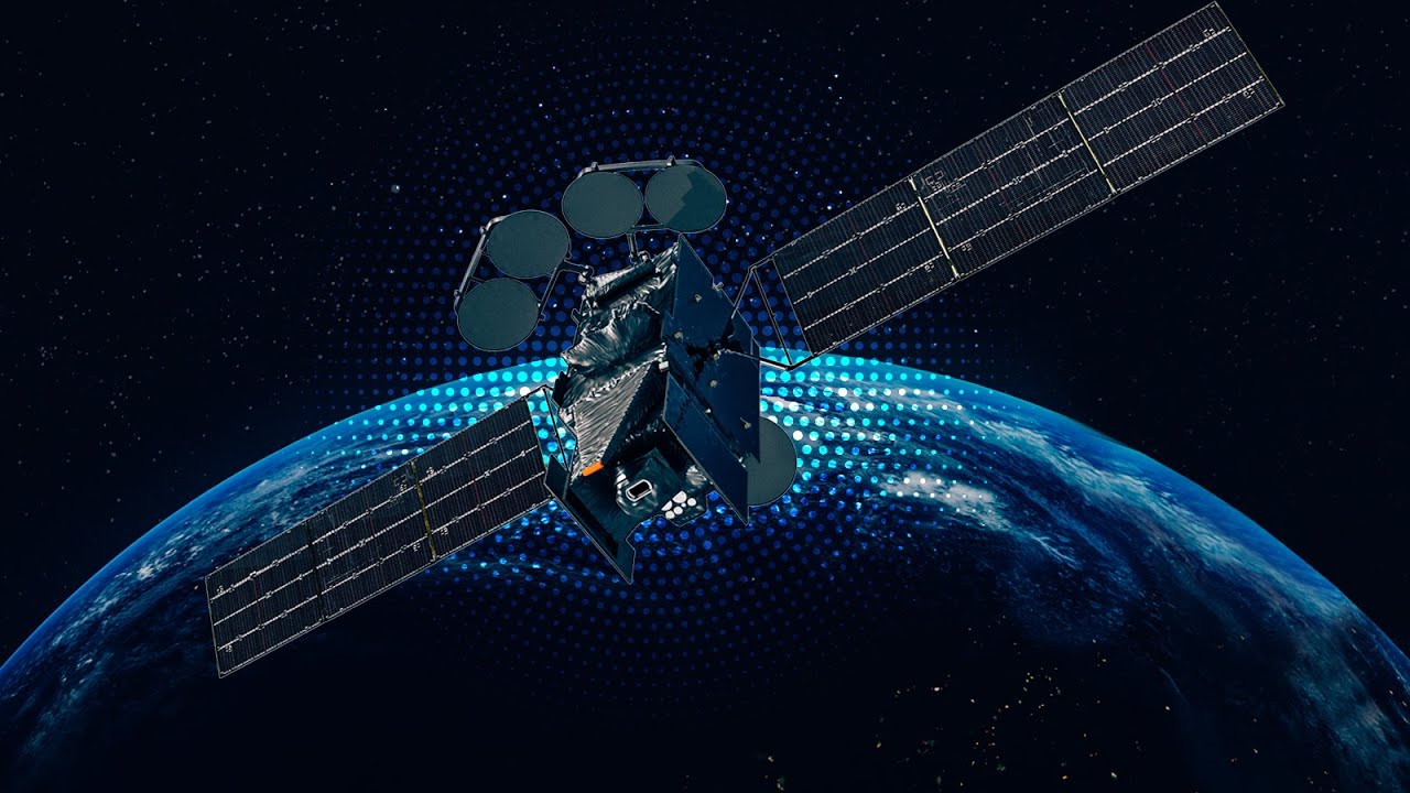
[00:28:34]And uh geostationary orbit uh is another orbit we can use for monitoring air pollution from space. And satellites in geostationary orbit or geo in short fly above earth equator as presented in this figure and uh they move from west to east exactly matching earth rotation. So GIO is ideal for satellites that need to stay fixed above a specific location. So uh satellites in geo can cover a large portion of earth and in this regard uh we have constellation of geostationary air quality satellites and the first instrument uh that was launched among these three was gems and it's it has been monitoring uh Asian air pollution since February 18 2020 uh and tempo for uh North American America was launched April 7, 2023.

[00:29:38]Uh and finally the third one, Sentinel 4 was launched July 1st this year and it's just nine days ago. So this is really exciting time for me and for for the field uh because we finally completed uh this constellation of geostation air quality con um um satellites. So we now recover these three major parts of the northern hemisphere and I'd like to describe uh more details about tempo. Now uh so tempo um provides hourly daytime air pollution measurements over North America. And the animation here shows one example of nitrogen dioxide measurements.

[00:30:25]And this um moving image represents uh the scan mirror position of the tempo instrument from east to west. Uh and that that's how this instrument scanned the domain here and tempo is NASA's first earth venture instrument and it was selected in 2012. uh in in a geostationary orbit.

[00:30:50]Tempo can continuously scan the continent with high temporal resolution and high spatial uh resolution. And the main advantage we have uh for tempo is that we have hourly coverage which low earth orbit instruments didn't have. Uh and baseline data products include nitrogen dioxide and formalhide which is one of the uh volatile organic compounds and ozone. And for the ozone part, we have two different products which I will cover later in this presentation.

[00:31:21]And this this figure shows uh tempo pixel size over Los Angeles. And because of the geometry, tempo pixel sizes are variable. Uh it's not a fixed value. And for this particular region, uh the area for each pixel is approximately 11 or 12 square kilometers. And the smallest pixel sizes are typically 9.5 kilometers uh over the bore sight location of the instrument. And it correspond to an area about the size of a small town.

[00:31:57]And to demonstrate how tempo can help understanding um the air pollution over North America, I brought this example.

[00:32:08]Uh so this map shows ozone air quality index for the same day as before July 6, 2025.

[00:32:16]And then here uh this region I uh I focused on the New York area.

[00:32:23]Uh and as you can notice there are some orange uh data points here uh which means uh sens sensitive groups and then orange and also green.

[00:32:35]uh and to understand the ozone production uh we need also NO2 and VOCC measurements. So I brought NO2 monitoring stations here.

[00:32:48]Uh so combining ozone and NO2 monitoring stations uh we can analyze uh where this ozone u originates and how NO2 concentrations change along with volatile organic compounds.

[00:33:06]But uh there are areas without monitoring sites and tempo can help uh filling this area uh as shown in this uh figure. Uh this is from the same date uh and 4:11 p.m. EDT and uh the tropospheric NO2 columns over this New York area uh is um has less uh gap between these uh pixels. uh although we have some uh um cloudy areas here where uh we we cannot measure accurately the NO2 column amounts. So basically we cannot see through clouds. So so um in in some studies we average monthly data of NO2 or annual data of NO2 to remove this gap in the data due to clouds. So that way we can have continuous map spatially and then assess the different pollution levels over the area and uh for the same day I moved to the Los Angeles area and also here we see orange spots and also yellow and also green. Uh this is for ozone air quality index and over the same area we have NO2 monitoring stations as well. uh and it is very nice uh that we can have this dense monitoring stations. Uh but with the te help of tempo we can also complete this map over this region. Uh and again these uh gray areas represent uh the the cloud uh presence. So um filtering out cloud is quite important for analyzing uh tempo data.

[00:34:57]uh and so far I've only presented one sin of uh Tempo NO2 tropospheric columns and uh as I mentioned before the main uh advantage that Tempo has is that it can provide hourly measurement of pollutants. So I brought an animation uh for the same day and you can see that this uh bar is moving representing different hours of the day and then the pollution changes over time. Uh so using low earth orbit uh we can measure NO2 over the same area and typically uh the overpass time is around 100 pm local time and we can add more information using tempo like this uh for the morning and also late afternoon.

[00:35:49]Um and tempo provides not only nitrogen dioxide but also formaldi concentrations. So this example shows simultaneous measurements of nitrogen dioxide and formalide over the Houston area for this selected date of August 2nd, 2024. uh and as shown uh in the previous slide there is dion variation hour hourly uh variation of pollutant um for NO2 and for malihide and they they present uh they um exhibit different spatial patterns. So by measuring these two different pollutants from space from the single instrument uh we can have uh information of NO2 for mali for the same spot and then analyze to understand better the ozone pollution.

[00:36:47]Uh and about the ozone itself. Um so o as ozone is dist distributed across the different layers of the atmosphere uh they have different sensitivity to the satellite measurements. Uh and it is well known that the stratospheric ozone layer blocks UV for us. Uh and there are three main uh wavelength ranges within the UV uh spectral range.

[00:37:17]uh and that they are UVC, UVB and UVA.

[00:37:21]So UVC is the shortest wavelength and it's the most sensitive to uh ozone and that's why we don't have much UVC exposure at the ground and UVB uh has less sensitivity to ozone and then UVA has the least sensitivity but they are all can be used to detect ozone. uh but since UVC uh doesn't reach the ground uh it's relatively hard to detect the bad ozone or ground level ozone. So we have total ozone product from tempo and pro profile products from tempo as well and they have different sensitivity.

[00:38:05]So here I I summarize uh the status of the tempo ozone products. So the total ozone product including uh stratosphere uh is now provisional validation status and here provisional means performance demonstrated and suitable for scientific publication. Uh but on the other hand we have also the uh ozone profile product which has been uh released uh to the tempo validation team only in limited sense. Um so the total sorry the ozone profile product is planned to be released to the public in late summer or fall this year after refining the algorithm because these two total and profile have different sensitivity.

[00:38:54]Uh and the ozone profile product will provide the troposate columns and here I brought uh the ozone profile u measurement result from another satellite. So the tempo ozone profile retrieval algorithm builds upon the heritage of the SAO low earth orbit algorithms and here OMI we we call it OMI uh is one of those satellite instruments uh where we apply the same algorithm as tempo. So this particular figure on the left shows the distribution spatial distribution of tropospheric ozone for summer 2013 and on the right here geoscam is one of the chemical transport model. So they show very consistent spatial patterns uh demonstrating the performance the good performance of the OMI satellite uh retrieval. So by applying very similar retrieval algorithm to tempo uh we will measure um tropospheric ozone and it it planned to be released to the public in late summer and fall this year.

[00:40:05]And finally uh this is my last slide. Uh and I I only covered ground monitoring of ozone and satellite monitoring of ozone but there are um other measurement platforms that we can use. So by using for example airborne measurements uh uh we can have more comprehensive understanding of the ozone production and also we have remote sensing instruments from the ground. So the uh measurement technique I described in this presentation from EPA uh is called in situ in our field but there are also remote sensing instruments uh from the ground and also uh we have airborne remote sensing instrument. So these field campaigns combined all ground, airborne and space-based observations using various measurements principles.

[00:40:59]So they provide comprehensive observations that are suitable for advancing our understanding of uh atmospheric dynamics and chemistry.

[00:41:09]So that's all uh I have for today and thank you very much for your attention.

[00:41:16]Thank you so much, Hung. That was fantastic. I feel like every time I talk with you all, I learn something more, which is exciting. Um, before I ask questions, I want to open it up and see if anybody here uh on the call with us has any questions they'd like to ask.

[00:41:33]And feel free to unmute yourself. Annie, go ahead.

[00:41:38]Hi, thank you. That was a great talk. Um I was wondering will the profile product be hourly and on the same spatial resolution as the tempo data?

[00:41:52]>> That's a very good question. Uh it will be hourly temporal uh resolution but the spatial resolution will be a little bit coarse than the other products. Uh because to enhance the signal we average four pixels. Um, so the pixel size will be slightly larger than the other products, but it will have the same temporal resolution.

[00:42:16]>> Thank you.

[00:42:21]>> Susan, do you have a question?

[00:42:22]>> Yeah, I had a quick question. Um, it has to do with the resolution and you were saying it, you know, it's fairly high resolution for this, but I'm wondering how how local is an ozone concentration? Is it um you know if you have a high ozone concentration because you live right next to a highway um you know if if there's a forest behind you is there going to be like a very different ozone concentration right there and how do you how do you measure that because I was noticing in the area where I live it looked like it was pretty good ozone but I'm finding maybe that's not the case.

[00:43:00]>> Yeah, that that's really a good question. So um as I mentioned the tempo pixel size is roughly 10 square kilometers >> uh and on the sub pixel level yeah there there should be variability of ozone uh NO2 and also VOCC um so we have this field campaigns with remote sensing airborne instruments and we can compare the spatial variability between the two satellite and airborne uh because aircraft measurements uh usually provide higher spatial resolution because it's closer to the ground and sometimes it can provide 500 mters of uh spatial resolution. Uh and when when we compared these two maps then we can notice there is sub pixel level variability.

[00:43:48]>> Uh so if we use only tempo measurements uh it will be very challenging to pick up those spatial variability within one pixel. But by combining with other uh platforms using airborne and ground, yeah, we can understand better the uh sub pixel level variability.

[00:44:06]>> That's great. Thank you.

[00:44:08]>> Thank you.

[00:44:11]>> Hi, I'm Mandy and I have a quick question. Um, you had mentioned, I'm not exactly sure which measurement, uh, but but you mentioned about how having cloud cover allows you to not be able to track certain, uh, ozone or other uh, levels. Um, and I was wondering how does that affect your readings if you have a area or region that has cloud cover for weeks on end which happens in our neck of the woods.

[00:44:45]>> Yeah, that's that's a really good question. So, uh, one of the level two products from Tempo is cloud. So, we have NO2 product, formaldi product, ozone product and also cloud product.

[00:45:00]And from this cloud product we retrieve uh the cloud cover for each pixel of tempo measurement. And the quantity represents the percentage of the cloud cover. And we usually use uh below 15% cloud cover. Um so if the cloud cover is below 15% then it means we can use it for research. But if it's higher than that uh then we we recommend uh users don't don't don't use those data because it has less accuracy. So if a certain region has cloud cover beyond 15% for a week then weekly average would not be sufficient uh to to assess the air quality over that region. Uh but if it's below uh 15% then we can still use the tempo data for that region. uh and and we can also average uh a longer time period uh to to secure uh clear sky pixels. So that that's usually uh how we uh secure data points uh to analyze different regions over North America.

[00:46:11]Thank you.

[00:46:13]>> That's a good question, Mandy. And I kind of have a follow-up question to that. I'm curious if the type of cloud impacts that as well. Like if it's a cumulus cloud versus a cirrus cloud, there's a bit more transparency of sunlight through each of those. So I'm curious if there's any information you have there.

[00:46:33]>> Yeah. Um we provide cloud fraction and cloud pressure. Um so uh by cloud pressure we can analyze how high this cloud is. uh but for from tempo uh we we do not provide uh specific types of clouds but that's really good point because um the cloud pressure is also important uh so when we calculate uh the vertical columns of uh trace gases uh we should convert the light path because it's usually slant for a particular region uh because the viewing angle from satellite is not vertical and this trendy from slend to vertical requires cloud information and in this process we consider both cloud fraction and pressure. So although we do not know if this cloud is uh cirrus or uh convection cloud uh we we do have information on pressure and the extent of the cloud cover. So we use those information to convert this light path.

[00:47:39]So yeah, that that's how we use uh this cloud information and it's really critical to the accuracy of trace gas retrieval.

[00:47:47]>> Thank you.

[00:47:54]>> I'm curious. I was kind of blown away by LA's numbers. You said it went from 065 to 007.

[00:48:03]Um how long did that take? Like once we get ourselves in these really bad situations, which we will continue to, and then we make an effort to clean it up, what's the time frame in terms of seeing a difference?

[00:48:27]So, um, yeah, let me go back to Sorry, I'm trying to find the proper slide.

[00:48:43]Um, >> so do do you mean the ch change in the ozone concentration over the LA region?

[00:48:59]Yeah, you had just mentioned that it was one of the regions that was most affected early on that kind of gave the United States a warning of smog and that it peaked at 6.

[00:49:10]>> Yes. Sorry, I just just found it. Yes.

[00:49:13]>> Um and I'm just wondering because now it's at 0.07. So like if it peaked at 0 65 in the 60 or mid50s when how long before it kind of came out of that? Like >> Loren, I'm going to point out that that's not at 007. 007 >> is attainment and LA is not in attainment.

[00:49:35]>> Got it. Okay.

[00:49:37]>> But it is better than it was, right?

[00:49:39]>> It's better.

[00:49:39]>> It's it's better than it was. Uh and I I don't have a time series of ozone concentration of uh over LA, but I I believe uh there there should be a time series of ozone measurement over those region. Uh yes. So I'm I'm sorry that I I I don't have a good answer to your question. Uh but it has been decreased and uh probably the EPA website should have this uh figure of time series uh decreasing ozone trend.

[00:50:09]>> Hey, I'll actually ask a follow up that I think will help Lorine process a little more because I know that during the pandemic Yes.

[00:50:16]>> some of these numbers changed drastically as well.

[00:50:20]>> You're right.

[00:50:21]Maybe you could talk about that a little bit and kind of like the time frame of like how quickly some of these things can be changed if we're working on it.

[00:50:28]>> Right. If we try.

[00:50:30]>> Yes, you're right. Um so during the pandemic um era we had decrease in not only in ozone concentration but also nitrogen dioxide and also VOCC's. Uh and then uh there there have been research uh that uh it bounced back um not not everywhere. Uh so depending on the extent of the anthropogenic activities we can have uh very quick change in air pollution. Um so I I believe the decrease of ozone uh could be um long-term effort but as Erica pointed out uh as we saw during the pandemic uh depending on uh how we control the emission and how we reduce uh the air pollution uh it can be happening uh in a shorter time period as well >> because it's my understanding from Caroline that NO2 is a pretty short-lived pollutant in the air.

[00:51:29]Correct.

[00:51:30]>> Exactly. Yes. So NO2 is lifetime because it reacts with sunlight. It's very short. Uh it's sometimes our level. Um so reducing NO and NO2 emissions um can impact the NO2 concentration in the atmosphere very quickly. Uh and since ozone is produced by NO2, although it has longer uh lifetime than NO2, uh since NO2 has been decreased, ozone can also decrease.

[00:52:04]>> Great. Thank you. Gives me some hope.

[00:52:07]Maybe >> air quality is definitely one we can fix if we put our ef our mind to it or at least make improvements on.

[00:52:18]Any other questions? We have time for maybe one more.

[00:52:32]All right. Well, we are just about at the hour. Um, this was fantastic. Thank you so much, Heang. It I, as I mentioned, I learned so much more today than I knew before. So, this was amazing, and we really appreciate you being here with us. And as a reminder to the community, this will go up on our YouTube channel. So this will be available uh for you to reference back to.

[00:52:54]>> Thank you very much.

[00:52:58]>> Have a great afternoon everyone.

[00:53:00]>> Thanks so much everyone. Thank you Han.

[00:53:03]>> Thank you.