







![CG M2 Pass Pack 💯🤩 Super Important [+PDF] 🎯 for 2022 Externals 🔥🔥🔥 6SEM CSE #vtu #2022 #CG #18CS62](https://i.ytimg.com/vi/HL-I7-5OB0s/hqdefault.jpg)



![Complex Analysis – II: [PART 4] Special Linear Fractional Transformations GGSIPU 2025](https://i.ytimg.com/vi/7d5RTcv6Xjo/hqdefault.jpg)







![[CA/Week 5] 5. Riemann surfaces, Introduction.](https://i.ytimg.com/vi/MegHwU8ywCA/sddefault.jpg?sqp=-oaymwEmCIAFEOAD8quKqQMa8AEB-AH-CYAC0AWKAgwIABABGGUgTShNMA8=&rs=AOn4CLCC3sV4NEXeFcGirF3JqWHtgsosnw)


The complex derivative extends the concept of differentiation to complex functions by representing it as a two-dimensional transformation that simultaneously encodes both the scaling factor (magnitude) and rotation angle (phase) of how small input changes affect output changes, unlike real derivatives which only capture one-dimensional scaling; this geometric interpretation reveals that complex differentiability implies powerful properties such as angle preservation (conformal mapping) and provides a unified framework for analyzing seemingly unrelated functions through their complex representations.
Complex Derivative Intuition: Geometry and Conformal Mapping
Added:Fundamentals of complex numbers, including polar representation and Euler's formula, which are essential for understanding geometric rotation and scaling.
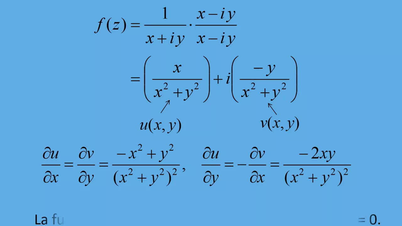
The definition of complex differentiability (holomorphy) and the algebraic formulation of the Cauchy-Riemann equations.
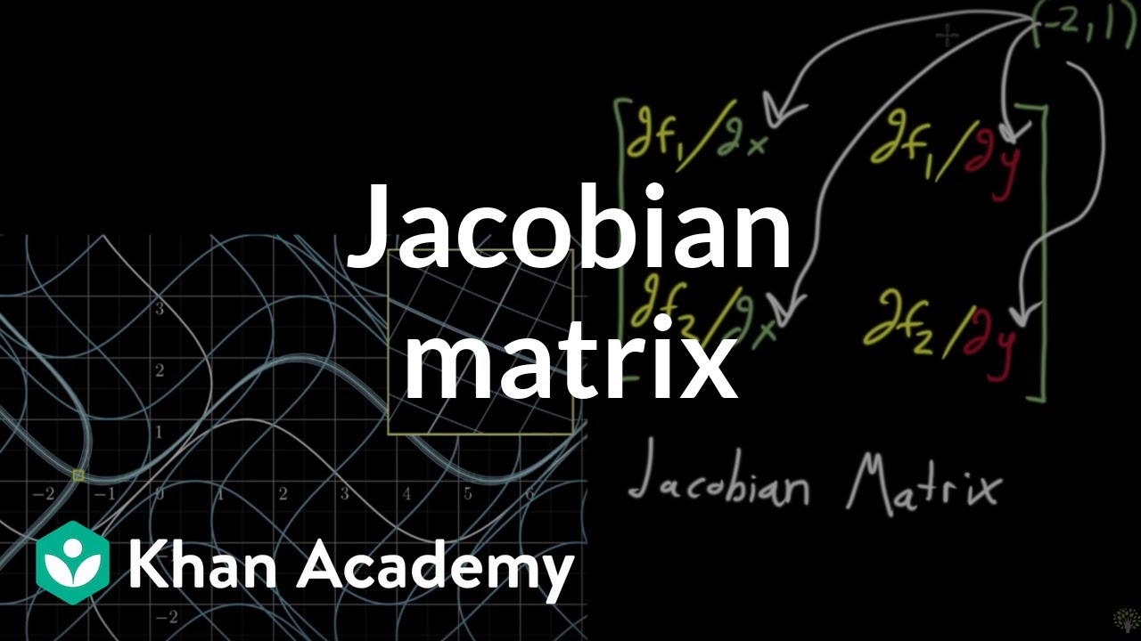
Basic multivariable calculus, specifically the concept of the Jacobian matrix and linear approximations of 2D real vector fields.
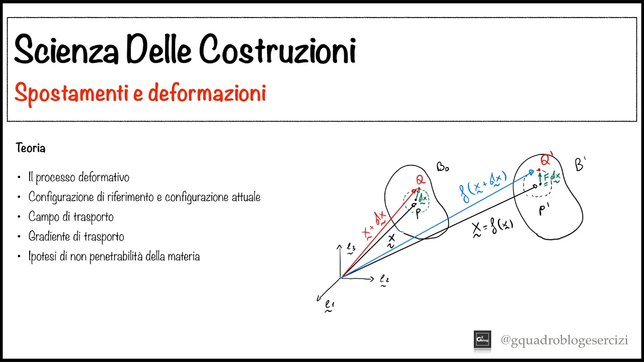
Geometric transformations in the 2D plane, such as translation, scaling, and rotation.
Applications of conformal mapping in physics and engineering, such as solving Laplace's equation in fluid dynamics, electrostatics, and aerodynamics.
The Riemann Mapping Theorem, which defines the conditions under which any simply connected open subset of the complex plane can be conformally mapped to the open unit disk.
The study of Möbius transformations, including their group properties and how they map generalized circles to generalized circles.
Introduction to Riemann surfaces to geometrically resolve and visualize multi-valued complex functions like complex logarithms and fractional powers.
221.1K views9.1Klikes14:54Original Release: 2020-11-05
this video was sponsored by curiosity stream home to thousands of documentaries and non-fiction titles for curious minds the complex derivative is much cooler than the regular derivative that we learn in calc one for real functions and that's because if you are told a function is differentiable like x squared or just a general f of x and then you're asked to say something else about that function just based off that information there's not much you could say that's too exciting i mean you could say it's continuous you could say there are no corners or cusps or anything like that and you can also say you know the the mean value theorem applies but past that kind of stuff again nothing too exciting with the complex derivative not the case if you know the complex derivative exists and maybe some other minor things about it you can answer some questions about some seemingly unrelated functions and we're going to get a glimpse of that later but first we've got to understand the intuition of what it means for a function to have a derivative of like 2 plus i now i know what you're thinking zack i didn't hear a word of what you just said because i was staring at that floating glow behind you i got that comment so much in the last video so i just want to actively say you can get this on stem merch this is available i'll put a link above and down below if you want to support the channel and get this for yourself but now i'm going to go off screen so we can kind of see how this all works now when thinking about just the regular derivative it can be more helpful to not think of it like the slope of the tangent at some point on the single two-dimensional plot but rather think of a one-dimensional number line for the input this is x and then one for the output and we'll use the function x squared so this is y if we put in one we get out one if we put in two we get out four three goes to nine and so on now to visualize the derivative at any point just place our input dot there i'll remove the other numbers so imagine we are very zoomed into x equals two and y equals four right now and then move the input a little to the right call that distance dx and look at how far the output traveled in response or d y in this case it moved four times further than the dx so the ratio or derivative at x equals two is four this is useful because everything moves in one dimension rather than like up and to the right with the tangent line when we move to equations with three variables it becomes a little more obvious why we do this because now the input can be any x comma y coordinate and that will map to a single z coordinate normally you graph that on a third dimension but separating the output z from the input space allows us to analyze the small changes better i can move the input in any direction on the plane choosing to move just a little to the right a small change in x yields an output that moves four times further so we say the partial derivative of z with respect to x at this point is 4.
if i instead move the input up a little bit then the output responds differently it moves twice as much thus the partial with respect to y at the same point is 2.
see this is a nice visualization because it easily allows us to see that output physically change in response to the changing input when dealing with a 3d plot that change can be harder to see but with complex functions there are four dimensions so now we have to use this method the input and the output space will both be two dimensional we can input any complex number like 2 plus i where you'll notice the y axis is just the imaginary component if we use the function z squared then the output is 3 plus 4i which can be solved with basic foiling and from here as we move the input around the output changes accordingly one thing that's really important to realize for later is that for any arbitrary input x plus i y we can simplify and split the output into its real and imaginary components so when we put in 2 plus i or 2 and 1 for x and y respectively then the real part comes out as 3 and the imaginary part comes out as four so three plus four i just like we got remember that but now the derivative of a complex function basically matches exactly that of real functions the function z squared has a derivative of 2z as expected but if the input is something like 2 plus i the derivative at that point is 4 plus 2y so what does that mean to have a complex derivative well it's really the same as what we've been seeing let's zoom into the input and output points and move the input just a little to the right we can call that whatever we want i'll say dz and note that the output moved about 4.47 times further that is the magnitude of the complex derivative it's how far the point 4 plus 2i is from the origin so that tells us just like before how much further the output moves compared to the input for any small change in any direction then if we call to the right 0 degrees then the output moved at an angle of 26.6 degrees roughly relative to that which is the phase of this complex number it's the angle from the positive x-axis and this is what the complex derivative tells us it reveals the ratio of the distances and the difference in the angles in regards to how the input moves versus the output meaning if instead the input moved at an angle of 45 degrees some small distance then the output would move still 4.47 or root 20 times further and an angle of 71.6 degrees which is still 26.6 more than the 45 for the input and from this you can see that if the derivative has no imaginary component like at z equals two plus zero i in this case then any small change in the input will result in the output moving in the same direction or the direct opposite here it's the same because the phase of the derivative is zero degrees thus the difference between the angles for the input and output is zero so they move in the same direction if the derivative were a negative real number then the phase would be 180 degrees and they move in opposite directions one consequence of this two-dimensional motion for both inputs and outputs is you have to be really careful when looking at whether a function is truly differentiable the first example most students learn is the conjugate function which reflects all inputs about the real axis two plus i goes to two minus i point five i goes to negative point five i and one goes to one basically all the real components stay the same while the imaginary components are multiplied by negative one this function is differentiable nowhere but it's continuous everywhere because at some point like 0.5 i if you move up a little bit the output will move down that same amount so in the opposite direction and this needs to stay consistent but if you move to the right the output will move in the same direction so it doesn't stay the same which means the derivative doesn't exist in more technical terms it means the limit doesn't exist the one which defines the derivative you don't think about this as much with real functions when you visualize the derivative at some point as the slope that the secant line approaches as the difference between your fixed point of interest and another approaches zero this can only happen in two ways approaching from the right or from the left with the complex derivative you have to think of one point sliding towards the other from all directions in the x y plane and make sure the limits all match if they don't then the function is not differentiable at that point now there's several interesting results that come from the complex derivative simply existing but one of my favorites would be this here if you have two paths in the complex plane that meet at some point where the angle between them we'll call theta then send them both through a function whose derivative exists and is non-zero at the intersection point like z squared the angle between the paths will not change it'll still be theta yes these resulting paths aren't even linear but that angle refers to the one between the tangent vectors for the two paths at the intersection point the angle you'd measure if you zoomed into the path until they looked essentially linear this angle preserving transformation is called a conformal map and it applies to all complex functions that are differentiable but non-zero at whatever your intersection point is here i'll do the same thing but for the function e to the z after that transformation again the angle is preserved in regards to the tangent vectors the transformation looks even better though when you do it for all the grid lines all the x equals a constant and y equals the constant lines because they all meet at right angles of course so if we map those to their outputs then those right angles should be preserved at all points where the derivative is non-zero i'll use z squared here and pay attention to like this intersection here after the transformation those output curves still meet at right angles and when you zoom in that becomes more obvious if we do the transformation with e to the z then same thing it looks messier but all those grid lines transform to either circles centered at the origin or diagonal lines and those all meet at right angles but there's something else that results directly from this remember from before we can represent a complex function in terms of its real and imaginary components now think about what will happen if we set this real part x squared minus y squared to a constant i'll choose two graph that curve on our input plane still the complex plane and map all those points through our function z squared well these are all the points where x squared minus y squared equals two so plugging any of those points into this here will yield an output of two for the real component therefore the output can only lie on this vertical line which has a real component of two and then i'll do the same thing for the imaginary component set that equation to a constant i'll choose one graph that and plug in all those complex coordinates to z squared when these go into the imaginary component we only get out one so all the outputs lie on this horizontal line which has an imaginary coordinate of one now regardless of how far the outputs extend along these lines we know if the original curves on the left intersect then the outputs on the right must intersect at this point here and at a right angle since angles are preserved through this conformal mapping then the two original curves must intersect at right angles which they do and this would apply for any constants that we choose so simply because z squared is differentiable and non-zero if we ignore the origin then we know this equation and this one known as the level curves must intersect at right angles outside of the origin for any constant values and if we plot those curves for many values of c1 and c2 we find that is exactly what happens i think that's really interesting because these don't seem related at all it would not be super easy to answer the question of at what angle does this curve intersect this one but once you realize these are the level curves that come from the simple function z cubed and separating that into real and imaginary components then you know oh yeah they must intersect at right angles since the derivative exists and is non-zero at those points and this does have applications in physics or engineering you can use conformal maps to move from a complicated domain to a simpler one do some analysis there and then map everything back so just another way complex numbers and complex analysis can and does apply to real world problems there are several other cool examples of how complex functions or derivatives almost magically seem to show up in physics applied math or engineering but i'm going to save that for a future video because i want to go into more depth but to continue exploring topics within applied math physics and engineering then i definitely recommend checking out curiositystream this video sponsor this here's a documentary called the secret life of chaos which actually discusses some of the beauty behind complex numbers like with the mandelbrot set then it also goes over how patterns and chaos apply to computer algorithms population growth and just the universe around us another series they have related to all this though is nature's mathematics which covers patterns and mathematical beauty found in nature like is the case with the fibonacci sequence so there's a lot to explore on this platform for the math and science enthusiasts out there curiosity stream is available on a variety of platforms worldwide and it only comes out to 299 per month but if you sign up by using the link below you'll get your first month's membership completely free so no risk in giving it a try and with this you'll have unlimited access to top documentaries that i'm sure many of you will enjoy and with that i'm going to end that video there thanks as always to my supporters on patreon social media links to follow me are down below and i'll see you guys in the next video
Up Next

42:44
Complex Numbers 2: Argand Diagrams, Modulus & Conversions
@jonahemmanuelofficial
123.2K views•2023-06-02

4:43
Elliptic Curve Cryptography Explained: ECC, ECDSA, ECDH
@PracticalNetworking
28.5K views•2024-10-21
22:59
Euler's Characteristic: Topology and Geometry Applications Explained
@zachstar
448.2K views•2019-09-13

6:00
The Mathematical Impossibility of Accurate World Maps
@Vox
23.3M views•2016-12-02
Related Study Plans & Knowledge Roadmaps
Structured learning paths in Mathematics
mathematics
Tensor Calculus: Vectors to Riemann Curvature
01Mathematical Foundations: Linear Algebra & Calculus
02Covectors, Dual Spaces, and Tensor Basics
03The Metric Tensor and Index Gymnastics
+ 2 more learning modules
40h5 modules
Explore Roadmap
mathematics
Gödel's Incompleteness: Logic, Proofs & Limits
01Introduction to Formal Systems & Hilbert's Dream
02Set Theory, Cardinality, and Cantor's Diagonal Argument
03Arithmetization and Gödel Numbering
+ 2 more learning modules
14h5 modules
Explore Roadmap
mathematics
Galois Theory: Fields, Groups & Solvability
01Foundations of Abstract Algebra: Groups & Fields
02Polynomials & Field Extensions
03Splitting Fields & Symmetries
+ 2 more learning modules
24h5 modules
Explore Roadmap
mathematics
Non-Euclidean Geometry: Models & Geodesics
01Euclid's Fifth Postulate and the Birth of New Geometries
02Hyperbolic Space and the Poincaré Disk Model
03Geodesics: Defining Straight Lines in Curved Spaces
+ 2 more learning modules
15h5 modules
Explore Roadmap