


![[Teoría descriptiva conjuntos] 38. Sigma-álgebra de Borel, funciones Borel](https://i.ytimg.com/vi/6fojakSjogE/maxresdefault.jpg)









![[ОВиТМ] Основы вероятности и теория меры (продвинутый поток) 7.](https://i.ytimg.com/vi/PBnyDHOpYLA/maxresdefault.jpg)





![Multidimensional Integration 16 | Lᵖ-Spaces [dark version]](https://i.ytimg.com/vi/p8j-QmL18XU/maxresdefault.jpg)
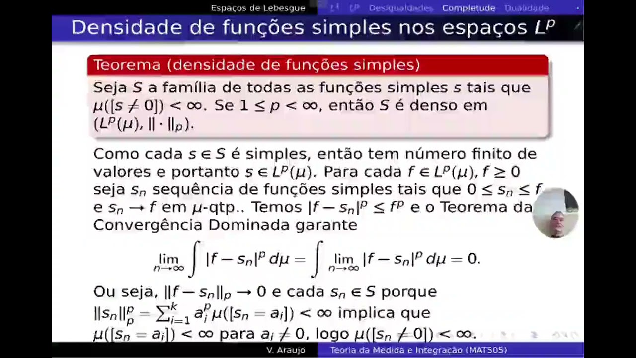
Simple functions, which are finite linear combinations of characteristic functions (indicator functions), can be used to approximate any measurable function pointwise and uniformly on bounded sets; this approximation theorem is fundamental in measure theory as it allows mathematicians to prove theorems about measurable functions by first proving them for the simpler class of simple functions.
Approximating Measurable Functions with Simple Functions | Measure Theory
Added:Definition of a measure space, including sigma-algebras and measurable sets.
The definition and properties of measurable functions (such as preimages of Borel sets being measurable).
The definition of simple functions as finite linear combinations of indicator functions of measurable sets.
Basic understanding of pointwise convergence and limits of sequences of functions.
The construction of the Lebesgue integral for non-negative measurable functions using the supremum of integrals of approximating simple functions.
Fundamental convergence theorems in integration theory, specifically the Monotone Convergence Theorem and Lebesgue's Dominated Convergence Theorem.
Lusin's Theorem and Egorov's Theorem, which provide deeper topological and uniform approximation properties of measurable functions.
The study of Lp spaces, including proof techniques that use the density of simple functions to prove properties of general integrable functions.
2.7K views64likes9:16Original Release: 2024-01-04
in this video we're going to talk about simple functions remember that if these kind of videos are helpful for you then you can donate on coffee to support the channel simple functions are a family of functions that are as the name says very simple and will be very useful to prove certain theorem only on this family instead of on a more general family of functions such as continuous functions or measurable functions to understand them we first have to understand a specific function called the characteristic function it's defined with this letter Kai and it's defined over a set e so we will take e as set let's say in our space X and now this function on some value X is defined as one if x is in e and zero if not it's very easy to see that Kai on some set e is measurable if and only if the set itself is measurable now these functions as I said are called characteristic or indicator functions well simple functions are just linear combinations of indicator functions and one important thing is that this linear combination will be finite so a function f is going to be an indicator function if it's of the form a n time Kai in N of X where we will say that n goes from one up to some capital n and the reason why we we take a finite linear combination is that we don't want indicator functions to take values plus infinity or minus infinity so we want them to always be finite and well that is obviously guaranteed when we add one only a finite amount of times now in this linear combination we can see a few things first of all we have this coefficient which just going to be any number and this number can be taken either on the real numbers or complex depending on whether we want our function to be real or complex function and then to Define these indicator functions what we need are sets E1 E2 and so on up to n in our Sigma alra so given a finite amount of sets in our Sigma algebra and some coefficients we can find form a simple function f but now why are these functions so important I mean they're extremely simple well they're important because of this next theorem this theorem says that we have a measurable space x m so a set and a sigma algebra a function that goes from that set to the zero Infinity so it's a positive function the same can be done if the function is negative that is measurable so if you don't remember some of these Concepts I recommend you check out our previous videos in the reproduction list what the theorem says is that there exists a sequence foren of simple functions that are increasing so each function is smaller than the next one and all of them are smaller than F and they're all positive that converge to F pointwise and uniformly on a set or F is bounded so why is this theorem useful well we know for example that continuous functions are measurable so what this theorem tells us is well any continuous function can be approximated pointwise or uniformly on a set where a function is bounded by simple functions and that is huge now we can take any theorem that is valid for continuous functions and instead of proving it for that huge family just prove it for simple functions this will be very helpful for us when we try and do integration theorems now the proof for the theorem is actually pretty ugly so what I'm going to do is instead of proving it because you can find the proof on any book Let's just try and draw how we can approximate a function the proof is actually building this sequence FN that will approximate our function so let's do that but with a drawing without all the mathematical notation that's a bit ugly in this case so let's say that our function f is something like this okay and let's say just to get a few numbers going that this number is two so this here will be one what we want to do is approximate this function f by simple functions well let's start with this number one we can just take a set like this so let's zoom in to see what's actually going on now we can see that there are a few regions where the function is greater than one and some other regions where it's smaller let's say that this is all above one so what we're going to do is Define a function a simple function as zero when the function is smaller than one and one where the function is greater than one so in this small interval the function is below the line so we will take zero then here it will be one all the way well okay here we have a simple function it's just this is going to be the set E1 this other one is E2 this E3 and this last one E4 and then the function is taking the value one or zero it's just going to be the sum of the indicator functions so this function let's call it 51 now let's build the second function what we will do is divide each of these two intervals into to 1/2 so here we have 1/2 and 3 over 2 now when we look at this first interval here the function is greater than 1/2 so it's going to take the value 1/2 now in the next one is greater than one so it's going to take the value one in this one it's greater than a half so it's just going to be 1 half but now in this case we have another separation here here so now we have the intervals E1 E2 E3 like before but this part changes we have E4 E5 and this last one E6 so now in E4 the function is again going to take the value one one because it's big greater than one but smaller than 3 over two and now in this region the function is greater than 3 over2 so it's just going to take the value 3 over two and now since here is below 3 over2 but above one it will take the value one well now this new function is going to be 5 2 and well my plot is not great because here I'm below two but if my function was oscillating a bit more or even not just oscillating but just growing then you can see how this sequence can be built so I'm just going to stop here because this is just a drawing but you can see that in the next step we would have to divide everything by 1 half again and do the exact same thing with it here but this drawing is going to be way more complicated so I'm just going to stop it there and you can follow building 53 and so on and this family of simple functions is very easy to see that they will converge pointwise to F and uniformly where the function f is pounded
Up Next
23:01
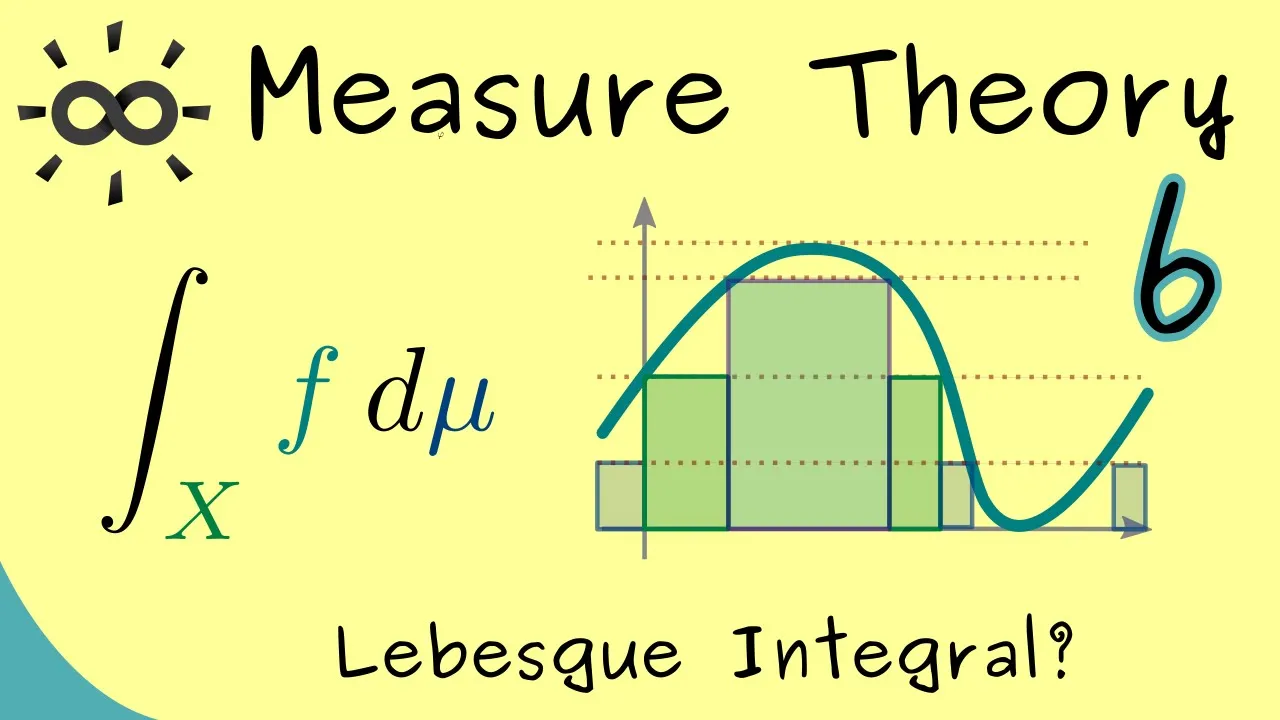
Measure Theory 6: Lebesgue Integral of Simple Functions
@brightsideofmaths
141.9K views•2019-09-29

4:43
Elliptic Curve Cryptography Explained: ECC, ECDSA, ECDH
@PracticalNetworking
28.5K views•2024-10-21

10:44
Fourier Series Introduction: The Big Idea Explained
@DrTrefor
387K views•2021-05-03

6:00
The Mathematical Impossibility of Accurate World Maps
@Vox
23.3M views•2016-12-02
Related Study Plans & Knowledge Roadmaps
Structured learning paths in Mathematics
mathematics
Tensor Calculus: Vectors to Riemann Curvature
01Mathematical Foundations: Linear Algebra & Calculus
02Covectors, Dual Spaces, and Tensor Basics
03The Metric Tensor and Index Gymnastics
+ 2 more learning modules
40h5 modules
Explore Roadmap
mathematics
Gödel's Incompleteness: Logic, Proofs & Limits
01Introduction to Formal Systems & Hilbert's Dream
02Set Theory, Cardinality, and Cantor's Diagonal Argument
03Arithmetization and Gödel Numbering
+ 2 more learning modules
14h5 modules
Explore Roadmap
mathematics
Galois Theory: Fields, Groups & Solvability
01Foundations of Abstract Algebra: Groups & Fields
02Polynomials & Field Extensions
03Splitting Fields & Symmetries
+ 2 more learning modules
24h5 modules
Explore Roadmap
mathematics
Non-Euclidean Geometry: Models & Geodesics
01Euclid's Fifth Postulate and the Birth of New Geometries
02Hyperbolic Space and the Poincaré Disk Model
03Geodesics: Defining Straight Lines in Curved Spaces
+ 2 more learning modules
15h5 modules
Explore Roadmap