A servo motor is a precision-driven motor that incorporates a feedback device (such as an encoder or resolver) to continuously monitor rotor position, enabling precise control of position, speed, and torque through a closed-loop system consisting of the motor, servo amplifier, and controller working together to adjust parameters in real-time.
How a Servo Motor Works: Technical Animation and Function Explained
Added:Deep Dive
Basic DC and AC motor fundamentals, including electromagnetism and torque generation.

Cómo el motor de Tesla humilló a Edison | Motor DC vs AC
7K
DC motors use brushes and commutators to change rotor polarity, creating friction, heat, and sparks that reduce lifespan. AC motors use rotating magnetic fields from stator electromagnets without brushes, making them more durable and efficient. DC current flows in one direction like cars on a highway, while AC current changes direction in cycles measured in Hertz (e.g., 60 Hz = 60 direction changes per second). Michael Faraday created the first electromagnetic motor in 1821 using liquid mercury to allow a rotating rod to close an electrical circuit without tangling cables.
Click to watch →

【심화반】 전기기기 06강(p.39~49)_1장 직류 전동기 ①(직류 전동기의 이론, 타여자, 직권, 분권, 복권 전동기)
246
DC motors operate on the interaction between magnetic flux and armature current, producing rotational force via Fleming's Left Hand Rule. When voltage is applied, current flows through the armature, creating a force that causes rotation. As the motor rotates, it cuts magnetic flux, generating back EMF (counter EMF) that opposes the applied voltage. Back EMF is calculated using E = (PΦZ/60a) × n and serves as a natural speed regulator. Torque (τ) is the rotational force measured in Newton-meters, calculated as τ = k × Φ × I_a. Angular velocity relates to RPM through ω = (2πn)/60. Power equals torque times angular velocity (P = τω). Alternative torque formulas include τ = (9.55 × P × Z × I_a)/(60a) × n. Torque units derive from force (Newtons) times distance (meters), giving Newton-meters or kg·m²/s².
Click to watch →

Unesp 2017 primeira fase - Resolução de Física
11.2K
This section covers electrostatics and electromagnetism. First, electric potential at a point is the algebraic sum of potentials from each charge: V = ΣkQᵢ/rᵢ. Electric field from a point charge is E = k|Q|/r², with direction away from positive charges and toward negative charges. In symmetric configurations, fields can cancel. Second, a DC motor consists of a rectangular coil in a magnetic field. Current flows from negative to positive terminal inside the battery, then through the coil. Fleming's left-hand rule determines force direction: thumb = force, index finger = magnetic field, middle finger = current. The side where force points inward is pushed down, creating torque that causes rotation.
Click to watch →

DC Motor में AC दी जाए तो क्या होगा ? | DC Motor on AC supply | AC Series Motor
171.5K
DC motors convert electrical energy into mechanical energy through electromagnetic forces. They are classified into three types based on winding connections: Series motors (armature and field in series), Shunt motors (armature and field in parallel), and Compound motors (combination of both). The torque production depends on the interaction between armature current and magnetic field. When current flows through armature windings, it creates a force that interacts with the magnetic field, producing rotational motion. The direction of torque is unidirectional in DC motors, meaning it always rotates in the same direction as long as current flows correctly through the armature.
Click to watch →

What on Earth Happened Part 10 Ewaranon - REUPLOAD
25.5K
Electric motors operate on electromagnetic principles: opposite poles attract, like poles repel. A magnetic field appears when current flows in a conductor—connecting a wire to a battery deflects a compass needle. Electricity creates a magnetic field, enabling electromagnets. In simple motors, a coil and permanent magnet create bouncing motion; balanced connections with proper polarity cause continuous rotation. Commercial DC motors use strong permanent magnets, large coils on armatures, and polarity control methods. The Faraday Effect demonstrates that electricity creates magnetic fields and vice versa—a 'chicken and egg' relationship. This bidirectional relationship is fundamental to understanding how electromagnetic luminaries like the sun and moon function, as magnetic fields can produce electrical currents and vice versa.
Click to watch →
Deep Dive
The conceptual difference between open-loop and closed-loop control systems.

Lec-2 Difference between Open loop and closed loop Control System | Control System|R K Classes|Hindi
27.1K
Open loop and closed loop control systems differ fundamentally in behavior, feedback mechanisms, and sensitivity. Open loop systems maintain consistent behavior without feedback, making them simple and economical but highly sensitive to external disturbances. Closed loop systems incorporate feedback paths with sensors/transducers, enabling adaptive behavior and superior disturbance rejection. While open loop systems are inherently stable, closed loop systems can be either stable or unstable depending on feedback type (negative feedback enhances stability, positive feedback may cause instability). The choice between them depends on application requirements for complexity, cost, and performance.
Click to watch →

Control System |State AE/JE 2021 Crash Course | free online Coaching |RSEB AE/JE Crash Course |L- 1
54.8K
Control systems are classified as open loop or closed loop based on feedback mechanism. Open loop systems lack feedback, making them less accurate, more sensitive to disturbances, and unable to reduce errors automatically. Closed loop systems use feedback to compare output with input, enabling automatic error correction, improved stability, and better disturbance rejection. Key differences include: open loop systems are more stable but less accurate, while closed loop systems are more complex but provide superior performance. The choice between them depends on application requirements for accuracy, stability, and disturbance rejection.
Click to watch →
CONTROL SYSTEM - 1 OPEN LOOP & CLOSED LOOP SYSTEM - TAMIL
61.1K
Open-loop systems apply input without feedback, while closed-loop systems use feedback to compare actual output with desired output. Open-loop systems have a simple input-to-output structure with no feedback path. Closed-loop systems include a feedback mechanism that continuously monitors output and adjusts control actions to minimize error. The key difference is that closed-loop systems can compensate for disturbances and maintain desired output despite external variations, making them more suitable for applications requiring precise control.
Click to watch →
![LAZO ABIERTO y LAZO CERRADO ✅ [Sistemas de CONTROL] #009](https://i.ytimg.com/vi_webp/CxGFoeJ7SD8/maxresdefault.webp)
LAZO ABIERTO y LAZO CERRADO ✅ [Sistemas de CONTROL] #009
161.7K
In control systems, an open-loop system controls a process based on pre-programmed instructions without using feedback from the output, making it simple and inexpensive but unable to compensate for disturbances or variations; conversely, a closed-loop (feedback) system continuously monitors the output using sensors, compares it against a desired setpoint, and automatically adjusts the control action to maintain the desired value, providing better performance and disturbance rejection but requiring careful controller tuning to prevent oscillations and instability.
Click to watch →

Stability of Closed Loop Control Systems
271.5K
Open-loop control systems do not use feedback to determine if the system has met its desired state; they don't observe or sense the output. In contrast, closed-loop systems use feedback of the output state to alter the input. The key difference depends on what you label as the reference signal and what is the output. A system can be considered open-loop if the reference doesn't depend on the output of the plant.
Click to watch →
Deep Dive
Pulse Width Modulation (PWM) and how electrical signals are used to command position or speed.

Essentials of PWM
36.1K
Pulse Width Modulation (PWM) is a technique for controlling power to electrical devices by rapidly turning the power on and off. The term can be broken down: 'pulse' refers to a signal that goes on and off, 'width' refers to how long the pulse stays on, and 'modulate' means to change. PWM converts analog signals (continuous values) into digital signals (on/off states) by representing the analog value as a percentage of time that the signal is on within a repeating cycle. This allows computers to control devices like solenoids and throttle positions by varying the duty cycle rather than using continuous voltage levels.
Click to watch →

What is PWM and how it works? | PWM signal explained | How to generate PWM Signal
139.9K
Pulse Width Modulation (PWM) is a technique that uses digital signals to control analog loads by rapidly switching power on and off at high frequencies, where the average output voltage is determined by the duty cycle (the ratio of on-time to total cycle time); this method is more efficient than using resistors for speed or intensity control because it minimizes power loss and heat generation, and can be implemented using circuits like the 555 timer IC or microcontrollers.
Click to watch →
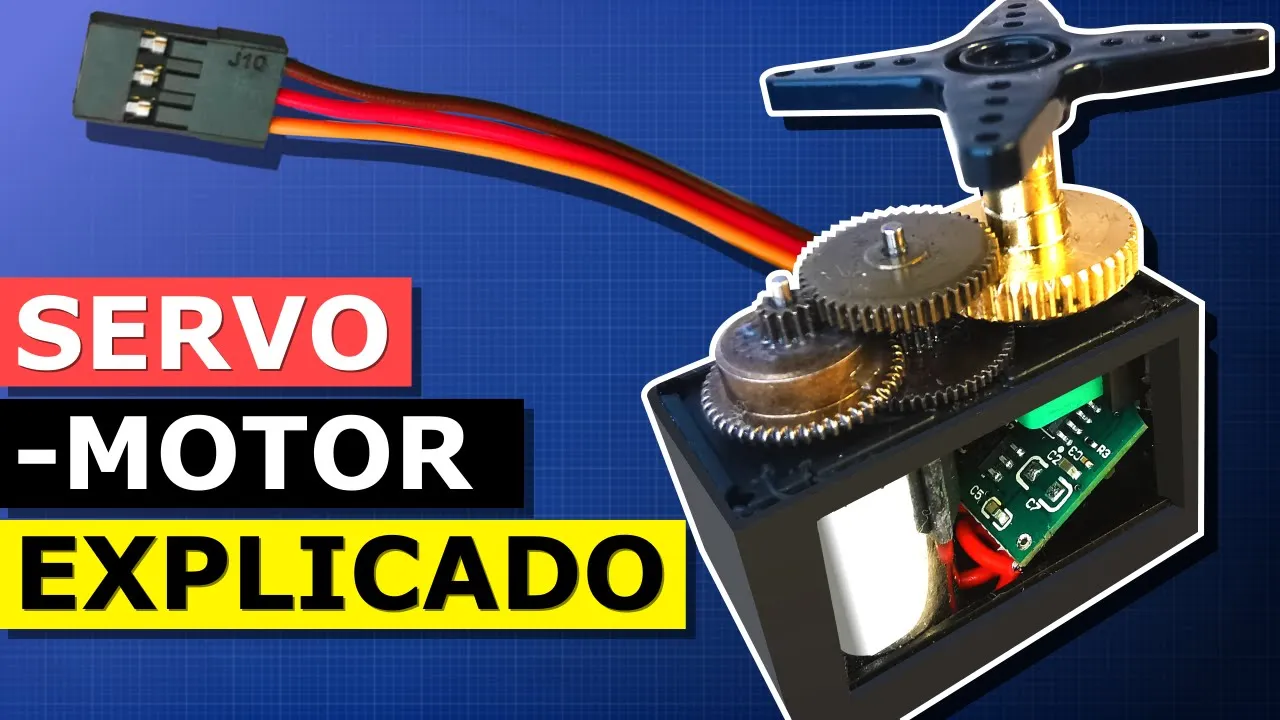
Servomotor Explicado
1.2M
Servomotors receive position commands through pulse-width modulation signals sent every 20 milliseconds (approximately 50 Hz). The pulse width determines the target position: wider pulses move the motor to one extreme, narrower pulses move it to the opposite extreme. Any position between these extremes can be achieved by adjusting pulse width proportionally. As long as the pulse width remains constant, the motor maintains its position; any change triggers movement toward the new position.
Click to watch →

Le soulèvement des machines, fabrication d’une tourelle Sky(pas)net - Road to partner (de fleurs)
24K
PWM (Pulse Width Modulation) is a signaling method where the width of electrical pulses carries information about desired motor position or speed. The signal repeats continuously, with pulse duration indicating how far the motor should move (e.g., 90°, 0°, -90°). The receiver interprets these pulse widths to control motor positioning.
Click to watch →
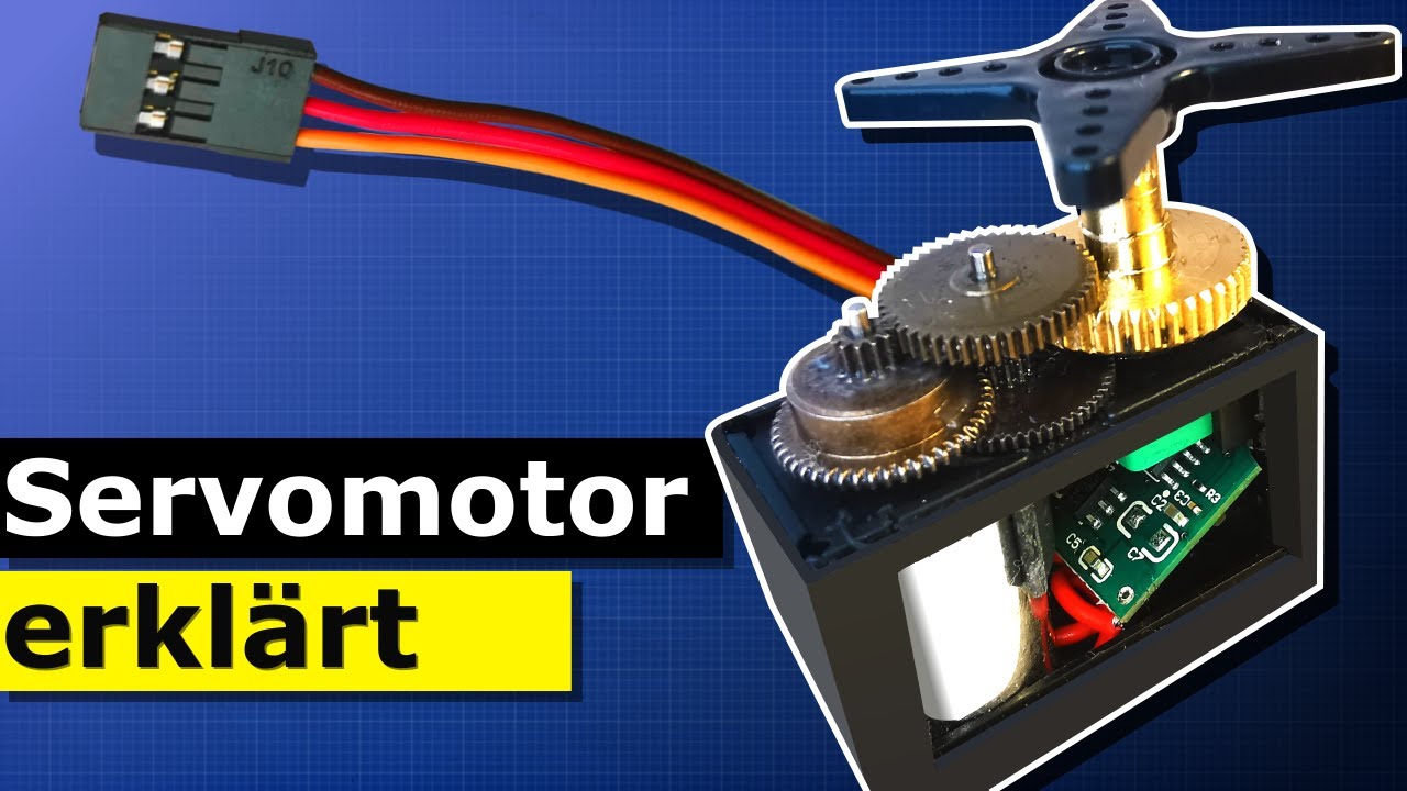
Servomotor erklärt
181.8K
Servomotors receive control signals using pulse width modulation (PWM), where voltage pulses are sent to the motor. The width of each pulse determines the desired position. These pulses are sent at regular intervals of 20 milliseconds (50 Hz frequency), meaning there are 50 pulses per second. The pulse width can vary to control the motor's angular position.
Click to watch →
Deep Dive
Basic sensor operations, specifically how potentiometers and rotary encoders measure mechanical position.
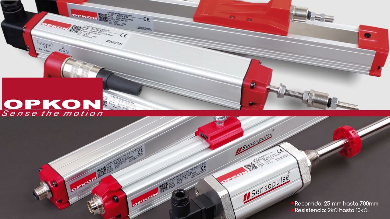
Funcionamiento de potenciómetros y encoders marca OPKON
1.1K
Linear position sensors, including potentiometers and encoders, measure the linear displacement of moving parts in industrial machinery by converting mechanical movement into electrical signals; potentiometers use variable resistance (typically 2kΩ-10kΩ) where resistance changes proportionally with axis displacement, while encoders generate quadrature pulse signals with resolutions as fine as 20-25 micrometers and travel ranges from 25mm to 50 meters, enabling precise position control in applications like CNC machines, hydraulic presses, and injection molding equipment.
Click to watch →
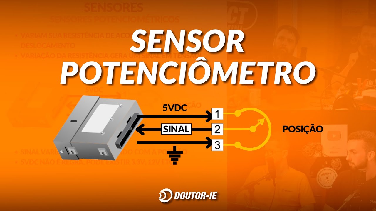
Como funciona o sensor de posição? (Potenciômetro)
415
Potentiometers are variable resistors that convert mechanical position into electrical voltage signals. They have three terminals: 5V power, ground, and signal output. A resistive track exists between power and ground, with a movable wiper that slides along it. The wiper position determines output voltage: near power terminal yields ~5V, near ground yields ~0V. In automotive applications, potentiometers serve as position sensors. The Throttle Position Sensor (TPS) measures butterfly valve position, outputting ~0.7V when closed and ~4.45V when fully open. Dual potentiometers with inverted signals sum to 5V, providing redundancy. The Accelerator Pedal Position Sensor (SPA) uses similar principles, with voltage ranging from ~0.5V (pedal released) to ~2.1V (fully pressed).
Click to watch →
4 _Mechatronics Sensors
600
Sensors detect system status by converting physical quantities to electrical signals. Transducers convert energy forms, classified by physical properties (mechanical, electrical, magnetic, optical) and output type (digital/analog). Linear guide systems convert rotational to linear motion using lead screws. Mechanical systems require position feedback due to wear and backlash. Potentiometers serve as position sensors by changing resistance based on slider position. The transfer function converts voltage to position: Output = (Supply Voltage × Measured Angle) / Total Range. For 10V supply and 350-degree range, at 82 degrees the output is 2.34V.
Click to watch →

¿Cómo funcionan los sensores de F1? | SoyMotor.com
40.2K
Potentiometer sensors measure linear or rotational mechanical positions by converting physical movement into electrical signals. Linear potentiometers have a sliding contact that moves along a resistive element, while rotational versions use a rotating shaft. In Formula 1, these sensors are applied to measure driver inputs such as accelerator pedal position, brake pedal travel, and steering wheel angle. The sensors connect directly to the car's ECU (Electronic Control Unit), sending real-time telemetry data to the garage. This allows engineers to monitor exactly what inputs the driver is making during testing and races, providing crucial feedback for setup optimization and driver performance analysis.
Click to watch →

MSFS 2024 | New User #3.2 | SPAD.neXt v0.9.24 + | Buttons and Switches
535
Potentiometers and rotary encoders require different configuration approaches than buttons. Potentiometers like the e-cam control have continuous values (0.5 in middle position, 0.05 increments) rather than discrete positions. SPAD.next maps these to analog axes (RZ axis) and uses rescaling to convert raw values (0-255 for 8-bit devices) to desired ranges (0-1). The system can rescale values to match the target variable's expected range, providing smoother and more realistic control. Range definitions allow limiting values to specific ranges, while rollover enables automatic wrapping at limits. The system supports scripted events attached to specific locations, enabling complex control behaviors.
Click to watch →
Prerequisite Knowledge
- Concept 01Basic DC and AC motor fundamentals, including electromagnetism and torque generation.
- Concept 02The conceptual difference between open-loop and closed-loop control systems.
- Concept 03Pulse Width Modulation (PWM) and how electrical signals are used to command position or speed.
- Concept 04Basic sensor operations, specifically how potentiometers and rotary encoders measure mechanical position.
Subsequent Learning
- Step 01Tuning PID (Proportional-Integral-Derivative) controllers for optimal servo response, overshoot prevention, and stability.
- Step 02Advanced feedback technologies, including absolute optical encoders and resolvers used in high-precision industrial environments.
- Step 03Multi-axis motion control and kinematics in robotics, automation, and CNC machinery.
- Step 04A comparative analysis of servo motors versus stepper motors and brushless DC (BLDC) motors for specific engineering applications.
Servo Drive Basics
AC Motor Design
Servo Drive Basics
0:02Playing Section
- 1
Defines servomotor as part of servo drive with rotor position sensors.
- 2
Explains system components: motor, amplifier, and motion controller.
- 3
Describes feedback loop for speed, torque, and precise positioning.
Open-Loop Stepper Motors and Sensorless Control
While servo motors excel in high-speed, dynamic applications due to their closed-loop feedback systems, they are often excessively complex and costly for many standard automation tasks. A key alternative perspective in motion control is the use of open-loop stepper motors. Steppers operate by moving in precise, fractional steps without requiring expensive feedback sensors (encoders) or complex control algorithms. For applications demanding high holding torque at low speeds, stepper motors offer a simpler, more cost-effective, and highly reliable solution. Furthermore, modern advancements in sensorless vector control allow systems to estimate rotor position mathematically, challenging the traditional servo's reliance on physical feedback hardware.
Deep Dive
Tuning PID (Proportional-Integral-Derivative) controllers for optimal servo response, overshoot prevention, and stability.

JMC Servo Tutorial Part 3 ► Grundlagen des Regelkreises an Bewegungssteuerungen
20.3K
A systematic PID tuning procedure ensures optimal servo system performance: (1) Start with current loop (usually pre-configured by manufacturer); (2) Tune speed loop by testing maximum settings; (3) Provide position setpoint for testing; (4) Input test trajectory (e.g., G0060 then G0061000) to observe position loop response; (5) Adjust P and I gains until system reaches setpoint without overshooting; (6) Configure acceleration and deceleration phases to balance responsiveness and stability. This methodical approach prevents oscillation and ensures the system responds appropriately to position changes while maintaining stability under various conditions.
Click to watch →

CONTROLE PID: como funciona e como ajustar o ganho PROPORCIONAL, o tempo INTEGRAL e tempo DERIVATIVO
23.7K
For proportional gain: disable integral/derivative, increase KP until instability, divide by 2 for stable starting point. For integral time: test values, decrease Ti until instability, multiply by 3 for stable starting point. For derivative time: increase Td gradually until instability, divide by 3 for stable starting point. After tuning, perform three tests: startup stability, disturbance response (process variable changes), and set point change response. Stability is more important than response speed. If overshoot is excessive, reduce proportional gain. If unstable, check if any action is set too high.
Click to watch →

Introduction to PID Control
111.2K
Increasing proportional gain (Kp): decreases rise time, increases overshoot, slightly affects settling time, reduces steady-state error, degrades stability. Increasing integral gain (Ki): decreases rise time, increases overshoot and settling time, eliminates steady-state error, degrades stability. Increasing derivative gain (Kd): minimal effect on rise time, decreases overshoot and settling time, no effect on steady-state error, improves stability if kept moderate.
Click to watch →

Understanding PID Controllers: Proportional-Integral-Derivative Explained
232.6K
This section covers advanced PID control concepts including derivative action, system response optimization, and practical implementation. The derivative controller adds a term considering how fast the error is changing, multiplying the rate of change (slope) by a constant (KD). If error decreases quickly (approaching goal too fast), the derivative term becomes a large negative number that dampens the response. When tuning PI controllers, engineers encounter overdamped responses (slow approach) and underdamped responses (overshoot and oscillation). The critically damped response achieves optimal performance—reaching set points quickly without overshooting. Manual tuning involves: setting Ki and Kd to zero, increasing Kp until oscillation occurs, then increasing Ki to correct steady-state offset, and finally adjusting Kd to eliminate oscillations. Modern PID controllers use code on microcontrollers. Key applications include automotive cruise control (originally researched for ship steering), manufacturing equipment, and reflow ovens for precise temperature control during soldering processes.
Click to watch →

PID Tuning with the Ziegler-Nichols Method: A Tutorial
377.6K
The Ziegler-Nichols method provides two empirical approaches for determining PID controller gains: the first method uses the step response curve's inflection point to calculate L (distance from origin to tangent) and T (vertical distance), then applies formulas (KP=0.9T/L, KI=1.2T/L, KD=0.075L); the second method involves increasing proportional gain until the system exhibits sustained oscillations at critical gain Kcrit and period Pcrit, then using formulas (KP=0.5Kcrit, KI=1/(1.2Pcrit), KD=0.125Pcrit) to determine controller parameters. Both methods are simple to implement but have limitations and work best for certain transfer functions.
Click to watch →
Deep Dive
Advanced feedback technologies, including absolute optical encoders and resolvers used in high-precision industrial environments.

Trasduttori di posizione: encoder (assoluto e incrementale) e resolver
4.1K
Position transducers convert mechanical position into electrical signals for control and monitoring applications. Optical encoders use photoelectric principles with alternating transparent/opaque disks to measure angular position, with absolute encoders providing unique position readings regardless of power loss (using Gray code for unambiguous readings) and incremental encoders generating pulses proportional to movement (requiring reference points for absolute position). Resolvers are inductive electromechanical transducers using electromagnetic coupling variation between primary and secondary windings, producing sinusoidal signals phase-shifted by 90° that vary with rotor angle, making them robust for high-temperature and high-vibration environments despite lower resolution than encoders.
Click to watch →

Sensores de Movimento e Posição | Introdução a Robótica #07
641
Resolvers offer significant advantages in industrial robotics: they have no electronic components in the sensor itself (reducing failure points), they are highly resistant to vibrations, and they maintain accuracy across temperature variations. These characteristics make them ideal for harsh factory environments. Optical encoders are position sensors that use light to detect angular position, consisting of a coded disk with patterns that block or allow light, light sources (LEDs), and photodetectors. They provide digital output signals and can be used for both rotational and linear position measurement. Absolute encoders provide complete angular position at any instant without needing to know previous positions and can recover position immediately after power loss without re-referencing.
Click to watch →

Capteurs |Résumés
16.6K
Position encoding technologies include incremental and absolute optical encoders. Incremental encoders use disks with tracks (A, B, Z) mechanically linked to moving elements, with optical emitters and photoreceptors. Tracks A and B are offset by 90° to determine rotation direction. Resolution is impulses per revolution; precision is 360° divided by number of intervals. Absolute encoders provide parallel outputs with each track having its own emitter/receiver system. Each angular position corresponds to a unique binary number, typically in Gray code to minimize transition errors. Resolution is 2^n where n is the number of bits; precision is 360°/2^n. Absolute encoders maintain position information even after power loss, unlike incremental types.
Click to watch →

Resolver
182.5K
A resolver is an absolute position sensor that uses electromagnetic induction between a stationary stator with three transformers (reference, sine, and cosine) and a rotating rotor to produce two output signals whose amplitude and phase relationship uniquely identifies the angular position of the rotor, making it ideal for high-vibration motion control applications.
Click to watch →
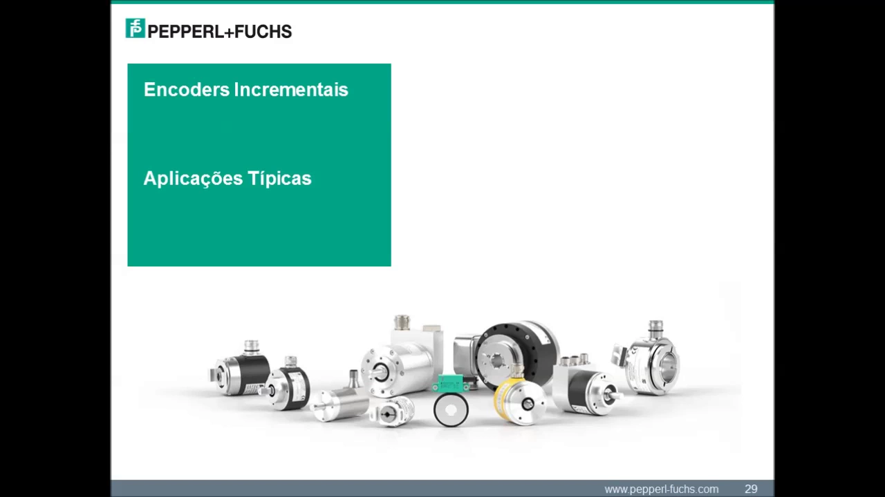
Encoders Rotativos
12.7K
Absolute encoders generate unique code values for each shaft position, maintaining position reference even after power loss. They are classified as single turn (one revolution, 16-bit max resolution) or multi turn (multiple revolutions, up to 30-bit resolution). Single turn encoders use optical multi-layer slotted disks or magnetic Hall sensors for robustness. Multi turn encoders add internal gear systems or magnetic sensors to count total revolutions. Output interfaces include network protocols (CANopen, DeviceNet, EtherNet/IP), synchronous serial for frequency inverters, analog outputs, and parallel interfaces. Applications span industrial tables, elevators, overhead cranes, paper machines, hydraulic presses, and port machinery.
Click to watch →
Deep Dive
Multi-axis motion control and kinematics in robotics, automation, and CNC machinery.
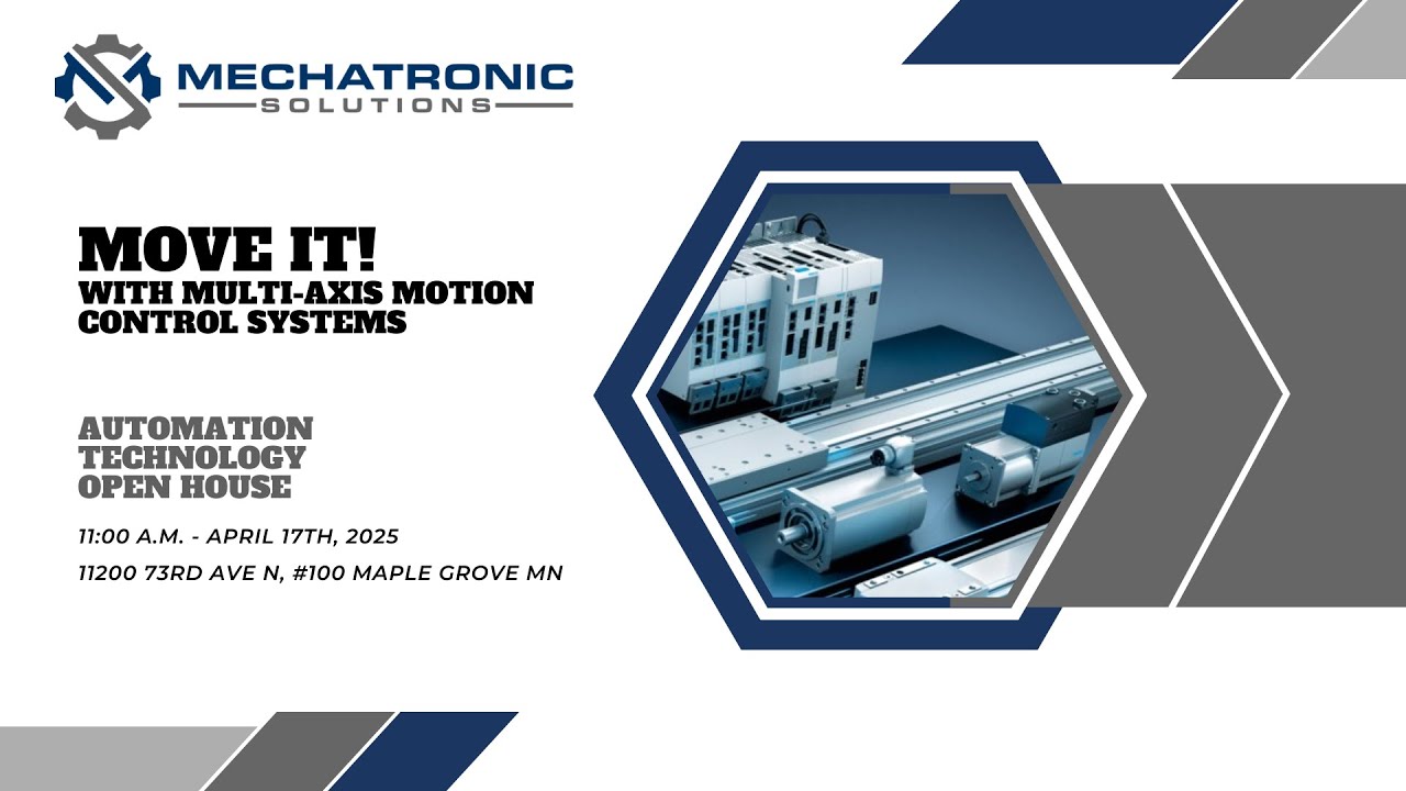
Move it! with Multi-Axis Motion Control Systems - Eric Rice from Festo | Automation Tech Open House
335
Multi-axis Cartesian motion control systems are modular positioning systems that combine linear actuators along X, Y, and Z axes to provide precise positioning in industrial automation applications. These systems offer significant advantages including decoupled payload and reach specifications (unlike articulated robots), consistent repeatability of ±0.1 to 0.15mm throughout the workspace, and straightforward safety guarding due to their fixed workspace envelope. The systems can be configured from standard catalog items ranging from single-axis systems to complex 3D gantries, with stroke lengths customizable to millimeter precision using belt drives or 100mm increments with ball screws. Applications span palletizing, pick-and-place operations, lab automation, and material handling, with options for adding rotary modules, pneumatic grippers, and integrated end-of-arm tooling.
Click to watch →

Motion Control 101 - Introduction
6.4K
CNC routers, laser cutters, and 3D printers share a common multi-axis motion control architecture consisting of X, Y, and Z axes for spatial positioning. The X-axis typically moves left-to-right along gantries, the Y-axis moves front-to-back, and the Z-axis controls vertical positioning. Some advanced systems incorporate additional axes such as a U-axis for rotary access, enabling cylindrical object machining. The video demonstrates this architecture across multiple machine types, showing how the same fundamental principles apply whether moving a cutting head, laser beam, or extruder nozzle. This commonality allows transfer of knowledge and components between different machine types.
Click to watch →
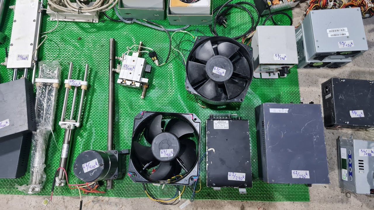
(15/9/2024) Các loại đồ tháo máy CNC 0975275636 0942453417
3.4K
Multi-axis motion control systems provide movement in multiple directions. The system includes four-axis movement (left-right, forward-backward) with a frame width of 8cm and height of 13cm. The system includes motor cables and sensor cables. These systems are essential for applications requiring complex motion patterns in automation equipment.
Click to watch →
HTTDServo_W15_NỘi SUY - MOTION CONTROL(P2)
2.8K
The video covers multi-axis motion control. Students learn how to control multiple axes of motion simultaneously, such as in robotic systems or CNC machines. The instructor explains that multi-axis control requires coordinating the movement of each axis to achieve the desired overall motion. Students also learn about the challenges of ensuring that all axes move in a coordinated manner to avoid errors or inefficiencies.
Click to watch →
3 2 2022 Lecture: Motion control for NC machine tools
101
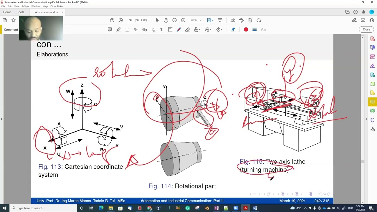
Multi-axis machine tools (like 5-axis machines) have additional rotational axes beyond standard X, Y, Z. The longer axis is assigned as X, the shorter as Y, with additional axes labeled accordingly. For complex machining, a global reference frame is established with Z-axis along the tool axis, X-axis along the horizontal plane, and Y-axis completing the right-hand rule. Local reference frames are calculated relative to the global frame for each point on the complex surface. This approach enables precise tool path generation for complex surfaces. The machine interprets G-code programs through its CNC unit, which reads program blocks and executes commands by converting instructions into actual machine movements, managing timing, velocity, and axis coordination.
Click to watch →
Deep Dive
A comparative analysis of servo motors versus stepper motors and brushless DC (BLDC) motors for specific engineering applications.
Какой привод лучше
247.4K
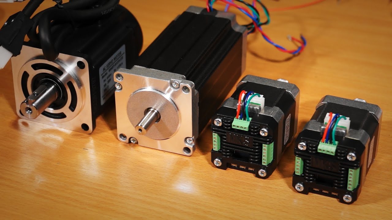
Servo motors outperform stepper motors in precision applications due to their ability to maintain constant torque across all speeds, eliminate resonance issues, and provide dynamic current consumption based on load, whereas stepper motors suffer from discrete stepping, resonance, constant current consumption regardless of load, and torque reduction at high speeds; modern servo motors have become more cost-effective than stepper motors of equivalent power, making them the preferred choice for precision machine tool applications.
Click to watch →

Servo Motor and Stepper Motor Difference
74.5K
Servo motors and stepper motors differ significantly in power supply (servo works on AC/DC, stepper only DC), control method (servo uses closed-loop with encoder, stepper uses open-loop), rotor poles (servo 10-20, stepper 200-400), rotational speed (servo 3000-6000 RPM, stepper 1000-2000 RPM), size availability (servo wide variety, stepper limited), lifespan (servo shorter due to brush replacement, stepper longer), complexity (servo complex, stepper simple), cost (servo expensive, stepper economical), performance (servo better under constant loads but hunts during positioning, stepper better under fluctuating loads), efficiency (servo highly efficient, stepper less efficient), and reliability (servo less reliable due to encoder failure risk, stepper more reliable). Servo motors are used in robotics, packaging machines, and medical devices, while stepper motors are preferred in 3D printers, semiconductor equipment, and security systems.
Click to watch →

MOTORS -The Secret Life of Components, a series of guides for makers and designers 11
164.7K
Brushless DC motors eliminate brushes entirely by electronically controlling coil energization. Coils mount on the stator while a permanent magnet rotor spins freely, removing brush wear limitations and potentially extending life indefinitely (limited only by electronics). They offer high starting torque, low noise, and are now widely available in consumer products including washing machines, drones, electric drills, and electric bikes. Servo motors contain encoders with fine-line discs that sensors read to track exact rotor position, enabling feedback-controlled positioning. Integrated servo motors combine motor, controller, and encoder in a single package, providing exceptional precision—returning to exact positions repeatedly. They excel in applications requiring extreme accuracy like robotics and precision automation, though they are more expensive than stepper motors. Smart motors represent an evolution of integrated servo technology, offering sophisticated control capabilities in compact packages.
Click to watch →
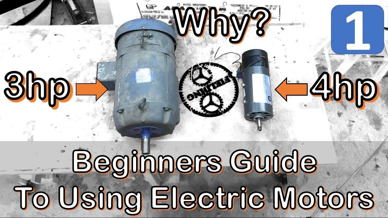
Ultimate Beginners Guide to Using Electric Motors for Makers and DIY Projects; #068
2.6M
Stepper motors provide exceptional positional precision, moving in increments as small as 0.9 degrees per step, making them ideal for industrial printers and CNC machines. NEMA ratings (17, 23, 34) standardize mounting dimensions rather than power specifications, enabling power upgrades through larger motors with compatible mounting patterns. Servo motors integrate brushless DC or AC synchronous motor technology with built-in encoders for closed-loop feedback, delivering high power and precise position/speed control for industrial applications. Brushless DC motors eliminate wearing brushes, offering longevity and performance comparable to three-phase AC motors, though they require specialized controllers and come in sensorless and sensored variants requiring different control approaches.
Click to watch →
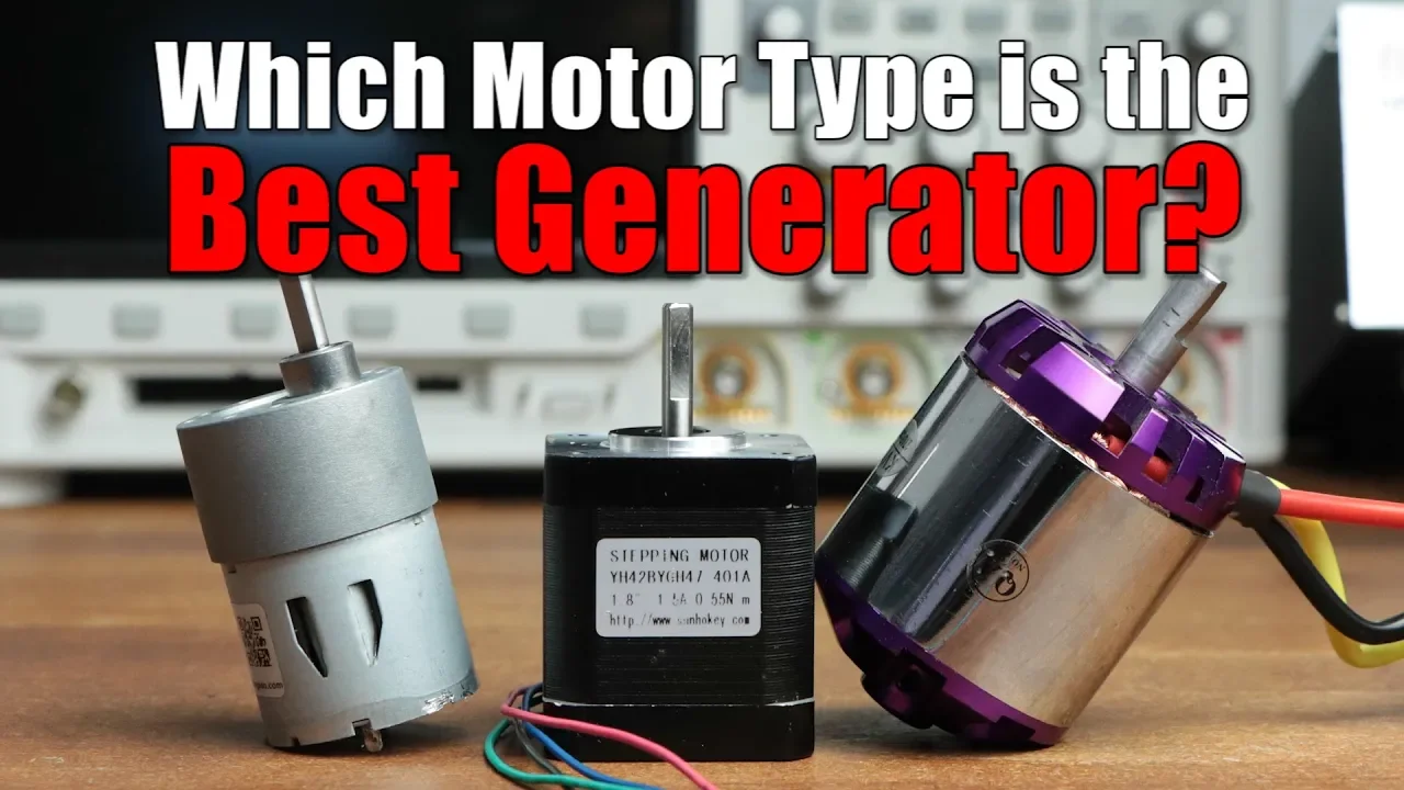
Which Motor Type is the Best Generator? || DC, BLDC or Stepper? (Experiment)
1.2M
In this experiment, GreatScottLab compares DC, BLDC, and stepper motors as generators by measuring their electrical output when mechanically rotated. The DC motor achieved approximately 4 watts of output power with 20-30% efficiency, the stepper motor also reached about 4 watts with similar efficiency, while the BLDC motor only produced minimal output at around 4% efficiency. The key finding is that fast-rotating motors like BLDC require gearboxes to increase RPM for effective generation, whereas stepper motors work well without gearing due to their design for lower RPM applications. DC motors are found to be the least suitable for generator purposes due to carbon brush wear and inefficiency at low speeds.
Click to watch →
Servo Drive Basics
AC Motor Design
Servo Drive Basics
0:02- 1
Defines servomotor as part of servo drive with rotor position sensors.
- 2
Explains system components: motor, amplifier, and motion controller.
- 3
Describes feedback loop for speed, torque, and precise positioning.
Open-Loop Stepper Motors and Sensorless Control
While servo motors excel in high-speed, dynamic applications due to their closed-loop feedback systems, they are often excessively complex and costly for many standard automation tasks. A key alternative perspective in motion control is the use of open-loop stepper motors. Steppers operate by moving in precise, fractional steps without requiring expensive feedback sensors (encoders) or complex control algorithms. For applications demanding high holding torque at low speeds, stepper motors offer a simpler, more cost-effective, and highly reliable solution. Furthermore, modern advancements in sensorless vector control allow systems to estimate rotor position mathematically, challenging the traditional servo's reliance on physical feedback hardware.
Basic DC and AC motor fundamentals, including electromagnetism and torque generation.
The conceptual difference between open-loop and closed-loop control systems.
Pulse Width Modulation (PWM) and how electrical signals are used to command position or speed.
Basic sensor operations, specifically how potentiometers and rotary encoders measure mechanical position.
Tuning PID (Proportional-Integral-Derivative) controllers for optimal servo response, overshoot prevention, and stability.
Advanced feedback technologies, including absolute optical encoders and resolvers used in high-precision industrial environments.
Multi-axis motion control and kinematics in robotics, automation, and CNC machinery.
A comparative analysis of servo motors versus stepper motors and brushless DC (BLDC) motors for specific engineering applications.
1.9M views14.4Klikes2:53@learnchannel-TVOriginal Release: 2017-12-28
This industrial robot needs a drive with particularly high demands.
Not only does the robot have to be able to accelerate and decelerate fast – also precisely positioning is required.
In fact, here is a three-phase servomotor installed.
In this video we will first clarify the term servomotor and servo drive in general, then the 3-phase-servo drive.
The servomotor is a part of a servo drive - whether brushless DC motor, synchronous or a robust asynchronous motor.
But one thing in common is the detection of the rotor position by a sensor.
This can be a resolver or an encoder – in this case you see an incremental encoder.
This sensor device gives feedback to a controller to keep for example the rotational speed or torque constant or to reach the target position as fast as possible.
A servo motor system includes the servo motor with its feedback device, a servo amplifier and a controller.
But how these devices work together?
The servo controller sends low voltage control signals for position, speed or torque to the servo amplifier.
Now these commands are amplified up to high power, which the motor can use.
The electrical pulses of a sensor are sent back to the amplifier.
This amplifier uses this information to control speed and rotor position.
The job of the servo motor controller, also named as the motion controller, is to close the loop on the system.
By constantly interchanging data with the servo amplifier, the motor parameters like torque, speed or position can be adjusted immediately.
Some manufacturers offer modules, which combine the controller and the amplifier.
So you would have fewer parts, fewer connections and a smaller footprint.
Talking about an AC servo motor you usually mean a 3 phase synchronous motor whose rotor field is excited by permanent magnets.
So you can get a very powerful and brushless motor of small size.
The stator winding produces a rotating magnetic field whose rotating speed and force is controlled by the amplifier and controller.
In order to position quickly, all these motors must have a low moment of inertia, which can be achieved by an elongated shape.
The functioning of a synchronous motor was already explained in another video of our learnchannel.
Please check our playlist.
Watch also our next videos!
Up Next

4:22
Raspberry Pi GPIO LED Control: Python Circuit Tutorial
@updowndown
120.8K views•2013-07-05

12:54
Triumph of Orthodoxy Icon: Byzantine Art & History Explained
@BenCallan
2.1K views•2024-08-06

9:49
FastAPI vs Flask vs Django: Choosing the Right Python Web Framework
@TechWithTim
302.5K views•2024-05-26

1:42
Game of Thrones Opening Credits: A Cinematic Analysis
@gameofthrones
46.3M views•2011-04-18
Related Study Plans & Knowledge Roadmaps
Structured learning paths in General & Interdisciplinary Studies
general-studies
Elevator Engineering: History, Physics & Cities
01From Hoists to Safety Brakes: The Dawn of Vertical Lift
02Hydraulic vs. Traction: The Engineering Physics of Elevators
03Modern Speed, Safety, and Algorithms
+ 2 more learning modules
12h5 modules
Explore Roadmap
general-studies
Rubber: Material Science, History & Geopolitics
01Origins of Natural Rubber & Mesoamerican History
02The Chemistry of Natural Rubber & Vulcanization
03The Geopolitics of the Rubber Boom & Colonization
+ 2 more learning modules
12h5 modules
Explore Roadmap
general-studies
Containerization: Evolution, Logistics & Trade
01Ancient Trade & Bulk Cargo: Amphorae to Barrels
02The Industrial Revolution & Cardboard Packaging
03The Containerization Revolution: Malcom McLean
+ 2 more learning modules
12h5 modules
Explore Roadmap
general-studies
Textile Tech: Evolution, Labor & Global Impact
01Pre-Industrial Textiles: Handloom & Cottage Industry
02Mechanization: The Spinning Jenny to the Power Loom
03The Factory System & Global Labor Transformation
+ 2 more learning modules
10h5 modules
Explore Roadmap