



![Espacio de Estados ► VARIABLES DE ESTADO 🤓 [Sistemas de CONTROL] #003](https://i.ytimg.com/vi_webp/BnCS3l3M09U/maxresdefault.webp)





![Stability and Eigenvalues [Control Bootcamp]](https://i.ytimg.com/vi/h7nJ6ZL4Lf0/maxresdefault.jpg)








![[SDII] Introducción al Control No Lineal](https://i.ytimg.com/vi/SwiHDa__AYo/maxresdefault.jpg)
Phase plane analysis is a graphical method for analyzing second-order non-linear systems by plotting the state variables (x1 and x2) against each other, where the phase plane trajectory represents the system's evolution over time and the phase portrait shows all possible trajectories from different initial conditions, enabling stability analysis and system design.
Phase Plane Analysis of Nonlinear Systems | Control Engineering
Added:Fundamentals of Ordinary Differential Equations (ODEs), specifically second-order linear and nonlinear differential equations.
State-space representation of dynamic systems, including state variables, state vectors, and state equations.
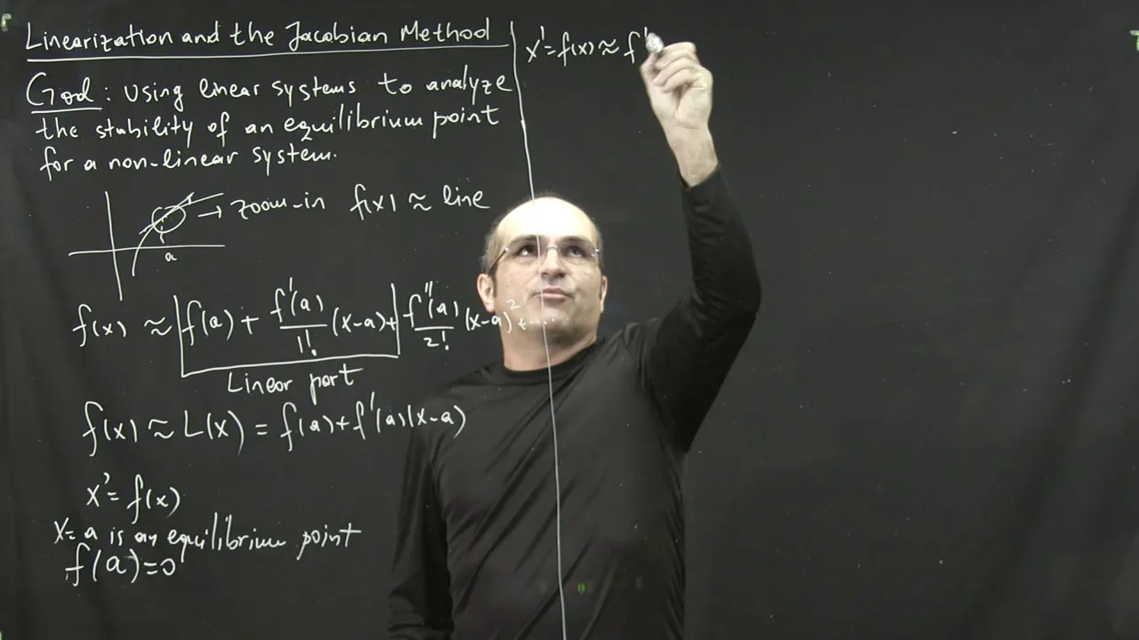
The concept of equilibrium points and the process of linearizing nonlinear systems using the Jacobian matrix.
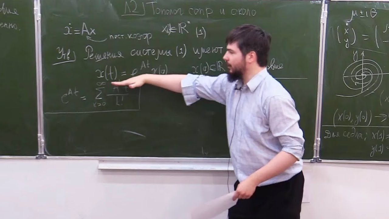
Stability analysis of linear systems, including eigenvalues, eigenvectors, and basic phase portrait classifications such as nodes, saddles, and foci.
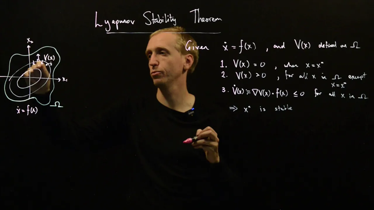
Lyapunov Stability Theory, including Lyapunov's direct and indirect methods for proving global and local stability.
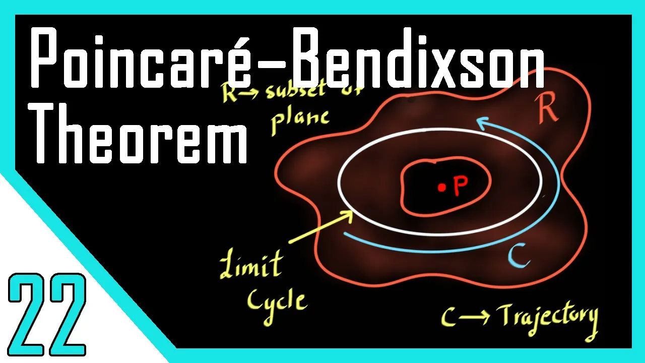
Advanced phase-plane phenomena, such as limit cycles, the Poincaré-Bendixson theorem, and bifurcation theory.
Describing Function Analysis, which uses frequency-domain methods to approximate and analyze nonlinear system behavior.
Nonlinear control design techniques, such as feedback linearization, sliding mode control, and backstepping.
128 views4likes26:49Original Release: 2021-08-18
in this session we will now start with the phase plane analysis uh so phase plane analysis is one of the methods of analyzing a non-linear system it's a graphical method to investigate the behavior of a non-linear system and also it helps us in designing the system parameters to meet the desired response of a system it's a graphical method so using this we can analyze a non-linear system as well as design the parameters for a particular desired response now one of the features of phase plane analysis is it is mostly applicable to second order nonlinear systems so we'll be having a second-order nonlinear differential equation uh and governing the system and from that we can actually be able to uh plot a phase plane uh so if we have a second order system that means we have two state variables x1 dot and x2 dot or you can say x1 and x2 so what phase plane and is it is the plot between x1 and x2 so ordinarily most most what we have the phase plane will be a plot between the states of this system and since it's applicable to only second order system there will be two states of the system so it will be a plot between x1 and x2 as far as higher order systems go it is very it becomes difficult for uh it becomes difficult to analyze uh or plot between number of state variables it is very complex to plot in a multi-dimensional plane and therefore uh phase plan analysis has been restricted to second order systems uh using that second order system analysis that can be extended to third order systems of fourth order systems but beyond that it becomes very complex because for an n-dimensional system for we cannot be able to actually plot in an n-dimensional plane and therefore this analysis has been in literature you'll see most of the analysis has been rested to second order non-linear systems only so what is a phase plane now it is basically a state space plane uh and whose xc's are the states of the system that is x1 and x2 and for at any instant of time we'll be giving the coordinates of the point in this plane and now the that means at any instant of time time will be varying from 0 to infinity at any instant of time x1 will be having a particular value x2 will be having a particular value and it can be traced onto this plane so as time varies from 0 to infinity this graph will change so it can be any type of graph i'm just showing that random graph here so as time t change from 0 to infinity the values of x1 and x2 will also change so at each instant of time the coordinates in this phase plane will give us will give us the point in the state space plane and uh the locus of these points that we are basically tracing in this phase plane is known as the phase plane trajectory so what's the phase plane trajectory it will be basically simply the locus of all these points in the phase plane that can be mapped onto this state space plane now for different initial conditions again now depending upon the initial condition of the system the trajectories will basically vary say for example this may be the trajectory for initial condition x 1 0 x 2 0 fine so this system was at this time uh the system starts from here because uh x one and x x naught y x one naught and x two naught are such the system uh starts from here and it will start tracing this path now you might have chosen a different initial condition that means say for example x1 x11 and x21 so the first point is located here so this will start tracing the path from this location so uh for different initial conditions of the system there will be different trajectories in this phase plane and the set of all these trajectories is actually known as a phase portrait one if we have only one plot it's known as a phase plane trajectory and a set of all these trajectories depending upon actually the initial condition of the system uh this that's actually plotted in this phase plane in the state space plane will be known as the face portrait uh say for example we have so for example we take a second order system consider the system y double dot plus 2 zeta y dot plus y equal to 0 and let the initial conditions of the system be x1 equal to the state of the system will be x 1 equal to y and its initial condition be y naught or i will simply write it as y naught and x 2 will be equal to y dot and y dot not i will say it is equal to zero so we have this second order system y double dot plus 2 zeta y dot plus y equal to 0 and i'm taking the two states of the system are x 1 and x 2 x 1 is y x 2 is y dot and in the initial conditions that i'm taking y naught and y dot of 0 i'm taking as 0 and so if we look at the solution of this equation number one k1 e raised power minus alpha t sine of beta t plus theta where k1 theta are constant and can be determined using the initial conditions so we have a second order system given here and the solution of the system is uh use this equation we have directly written the solution here uh we'll actually be looking at how to obtain the transfer function model later uh now if we look at the roots of the system the roots of equation 1 actually in terms of alpha and beta will be minus alpha plus j b and minus alpha minus j beta fine now if we are to plot x1 and x2 t what happens is this will be the plot of x1t x1 with respect to time t and this will be the plot of x2t with respect to time t now what is phase plane it will be the plot of x1 and x2 with respect to each other now if we had to plot between x1 and x2 uh x1 we had said it will be the initial condition of x1 will be x1 naught and x2 that's y dot will be zero so it is starting somewhere here so this is x1 this is x naught 0.
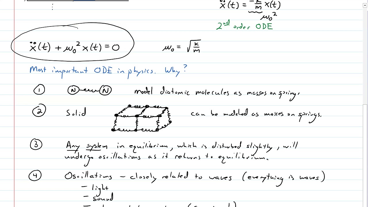
so it starts here x1 and x2 both are slowly decreasing and it will ultimately end up at the origin of the system so this is the trajectory that this equation will be following this is the plot between x1 and x2 so this curve here actually represents uh a log logarithmic spiral and that is actually merging towards the equilibrium point of the system now origin of the phase plane is actually the equilibrium state of the system so if origin of the system origin of the phase plane will not be the equilibrium point we shift the origin towards the equilibrium point so that always this origin will be the equilibrium point of the system fine so determine we have to also first of all determine the equilibrium point so if it is equivalent point is zero zero so that means that's fine if the equilibrium point is say for example two comma zero uh we'll shift the origin towards two comma zero so that our origin uh now how we have shifted the plane so that our origin again becomes equal to zero zero uh now what we have done so far is simply uh we have seen what a phase plane is it is a plot between two states of a system x1 and x2 y2 states because phase plane is only applicable to second second-order non-linear systems and locus of all those points that you will be tracing as time varies from 0 to infinity in the phase plane is known as a phase plane trajectory but depending upon the initial condition of the system you you for the same system you'll be having a number of trajectories and a set of all those trajectories is known as a phase portrait we took an example of a simple second order uh system and for the second order system x1 equal to y x2 equal to y dot now this equation here this is actually the solution of a second order linear system and that solution you actually already found for these roots fine these are these are two roots that are located here and here that actually correspond to uh and under that response so for that res for that you already know that y t is equal to this thing uh where k and theta represent here two constants that can be determined from the initial condition of the system so we are starting actually with the uh linear system you have therefore the plot of x one t you have the plot of x x2t you can determine these two plots for the system now if we want to plot between x1 and x2 you'll see the plot will be something like this so this is the phase plane of this linear system that we have just obtained phase plane portrait and this phase plane shows us we are obtaining a logarithmic spiral that emerged from the initial condition of the system and ends up at the equilibrium point of the system point so this is what the phase plane is now the main thing here is that it is restricted to second order non-linear systems only now let's take another example x double dot plus x equal to zero so we have a nonlinear system so this this equation actually represents the behavior of a mass spring system all right so x double dot plus x equal to zero uh you have a mass spring system like this so what we are considered assuming here is that let us assume that mass is initially at rest at any length x naught fine so we have x double dot plus x equal to zero uh so we can find out the solution of this equation this is simply d2x by dt square plus x equal to zero so you can actually apply the laplace on uh both sides so if we apply the laplace here so you'll be having s square x of s x double dot plus x equal to 0 d2 x by dt square plus x equal to 0 is applying the laplace to this equation uh laplace of d to x minus s x naught minus x derivative not plus laplace of x of s equal to zero which implies uh this here is x naught this will be zero therefore s square x of s minus x naught of s plus x of s equal to 0 this is 0 because we are assuming that the mass is at rest so x derivative of 0 so velocity will be 0 initially x of s common uh so you can say this is x of s equal to x naught of s x naught s divided by s square plus 1 fine so we have x of s equal to x naught into s divided by square plus one this is x of s so that means x t will be equal to laplace inverse of s by square plus 1 that is cos of t so if this is x t that means actually this x 1 t x 2 t will be x 1 t dot product of x 1 t that is minus x naught sine of t fine so we have a differential equation x double dot plus x equal to zero apply laplace to both sides you will get s square x s minus s x naught minus x dash of zero plus x of s equal to zero now as far as the initial conditions are concerned x 0 is equal to x naught this length l that is actually where the mass is resting and x dot of zero this is x dot of zero uh the since it is at rest the velocity will be zero so this we will be putting it to equal to zero so s square x of s minus x naught s plus x of s equal to zero x of s common so you'll get getting x naught as divided by square plus one s divided by x square plus 1 is actually cos of 80 a is 1 here so x 1 t is x naught cos t so x 2 t is minus x naught sine t so we have x 1 t x 1 equal to cos t x 2 equal to minus x naught x naught minus x naught sine t so if x naught say for example is equal to 1 x 1 will be equal to cos that means it is actually something like this this is x1 with respect to time t and what is x2t uh x2 is minus x naught sine t x naught we are assuming it is 1 so minus sine t means it will be something like this so we can also plot x1 t with respect to x2t or we can scan and mult square both these two terms and add them together so x1 square plus x2 square is equal to x naught square cos square plus sine square cos square plus sin square is equal to one so x one square plus x two square is equal to x naught square uh which is actually uh the equation of a circle so when will be plotting x1 and x2 so depending upon the value of x naught which x naught naught will be the radius of the system so we'll be getting different curves so we can get this curve uh depending upon say for example x naught equal to one we'll be getting this curve depending upon say for example x not equal to 1.5 so we'll be getting this curve this is a plot now between x1 and x2 and x naught in this case is say for example equal to 2.
so we have got an equation this equation represents the equation of a circle x1 squared plus x2 square equal to x naught square where x naught is the radius of this circle so for different x naughts there is actually different initial conditions so wherever the mass is located so if it is located at this position or if it is located at this position initially or if it is located at this position so whatever is the initial location of the mass accordingly we will be getting the phase portrait of the system that is actually the plot of x1 with respect to x2 of the system so this is so far what we have seen only the basics of phase portrait now what we have to do is we have to find out how to plot a phase portrait so there are uh two methods analytical method and isoclient method that we'll be studying that are used for plotting the phase portrait of any system and also we need to understand the stability how to check the system stability using the phase portrait how this phase portrait here actually tells us whether the system is stable or not fine also note the direction of motion of these particular portraits so that will be all for this session in the next session we'll start with understanding the analytical how to check the analytical solutions of facebook rates
Up Next
10:52
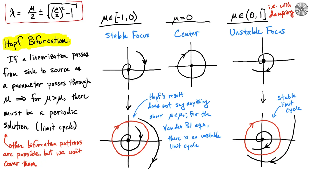
Limit Cycles & Bifurcations | Van der Pol Equation Explained
@justinruths9590
30.1K views•2019-04-09

4:43
Elliptic Curve Cryptography Explained: ECC, ECDSA, ECDH
@PracticalNetworking
28.5K views•2024-10-21

10:44
Fourier Series Introduction: The Big Idea Explained
@DrTrefor
387K views•2021-05-03

6:00
The Mathematical Impossibility of Accurate World Maps
@Vox
23.3M views•2016-12-02
Related Study Plans & Knowledge Roadmaps
Structured learning paths in Mathematics
mathematics
Tensor Calculus: Vectors to Riemann Curvature
01Mathematical Foundations: Linear Algebra & Calculus
02Covectors, Dual Spaces, and Tensor Basics
03The Metric Tensor and Index Gymnastics
+ 2 more learning modules
40h5 modules
Explore Roadmap
mathematics
Gödel's Incompleteness: Logic, Proofs & Limits
01Introduction to Formal Systems & Hilbert's Dream
02Set Theory, Cardinality, and Cantor's Diagonal Argument
03Arithmetization and Gödel Numbering
+ 2 more learning modules
14h5 modules
Explore Roadmap
mathematics
Galois Theory: Fields, Groups & Solvability
01Foundations of Abstract Algebra: Groups & Fields
02Polynomials & Field Extensions
03Splitting Fields & Symmetries
+ 2 more learning modules
24h5 modules
Explore Roadmap
mathematics
Non-Euclidean Geometry: Models & Geodesics
01Euclid's Fifth Postulate and the Birth of New Geometries
02Hyperbolic Space and the Poincaré Disk Model
03Geodesics: Defining Straight Lines in Curved Spaces
+ 2 more learning modules
15h5 modules
Explore Roadmap