























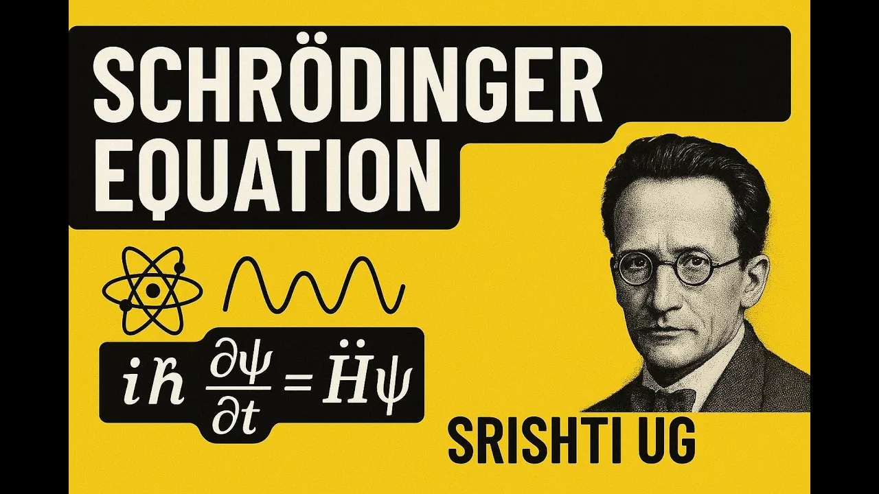


The Schrödinger equation is the fundamental equation of quantum mechanics that describes how quantum systems evolve over time; it states that the imaginary unit times Planck's constant over 2π multiplied by the partial derivative of the wavefunction with respect to time equals the Hamiltonian operator acting on the wavefunction, where the Hamiltonian is the sum of the kinetic energy operator (negative h-bar squared over twice the mass times the second spatial derivative) and the potential energy operator. The time-independent Schrödinger equation is derived using separation of variables, assuming the wavefunction can be written as a product of a spatial function and a temporal function, leading to the equation Hψ = Eψ, where E represents the eigenenergy of the system and determines the time evolution of the wavefunction through the exponential factor e^(-iEt/h-bar).
Schrödinger Equation Explained: Hamiltonian & Time-Independent Derivation
Added:In the two previous tutorials we learned about a number of quantum operators as well as the wavefunction. We also learned how to calculate expectation values, which represent the way to determine the results we can expect when we measure specific variables for a quantum system. Now it’s time to put it all together, so that we can revisit the Schrodinger equation in more depth. In one of the first tutorials in this modern physics series, we displayed the Schrodinger equation in roughly the following form, although we barely discussed it at all, since we were not equipped to do so. Now we can read this properly as i times h bar times the partial derivative of psi of x and t with respect to time, being equal to the Hamiltonian operator acting on psi of x and t. So we will now be more precise in having psi depend on both position and time. The only thing in this equation that remains unfamiliar at this point is the Hamiltonian operator. We know what operators are in general, so let’s define this one. The Hamiltonian operator has two components. There is a kinetic energy operator, T, and a potential energy operator, V, and the Hamiltonian operator is the sum of these two operators. In the previous tutorial, we defined the kinetic energy operator, and found that it was equivalent to this expression, negative h bar squared over 2M times a second partial derivative with respect to x, so let’s go ahead and make that substitution now. The potential energy operator is a little trickier, as it will depend on what type of potential we have, so let’s just leave that as it is for the time being. With the Hamiltonian operator defined, let’s now plug this into the Schrodinger equation in place of H. And that leaves us with the explicit expression of the Schrodinger equation. So, we finally have this important equation well-defined with terms that we understand, but what does the equation mean? Well, one straightforward way to find meaning in the Schrodinger equation is to think of it kind of like Newton’s second law for quantum mechanics. For a given set of initial conditions, which can be written down in the initial wavefunction psi of x and t at t equals zero, the Schrodinger equation can tell us how the system will evolve with time. That is, what future iterations of psi of x and t will look like. This is precisely the way that knowing the initial values for position, velocity, and acceleration with regards to a classical particle, and being aware of any forces acting upon the particle, we can determine what any of these parameters will be at some future time. But in the tutorial following this one, we will use the Schrodinger equation in a way that does not really have a counterpart in classical physics. We will use it to find what the wavefunction looks like for a static condition. This would be like saying that we will use Newton’s equation to find out what a tennis ball looks like, which sounds absurd. But in quantum mechanics, objects are described by wavefunctions, which, as we saw, are not point-like entities. The spatial distribution of quantum objects is determined by the boundary conditions of the system at hand, and it is those conditions that constrain the actual physical shape of the probability density function that governs any quantum object, as we have discussed previously.
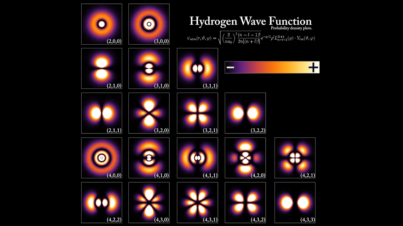
This is a really abstract concept, but grasping this idea will allow us to really understand things like atomic orbitals with exceptionally greater depth than before. We have to internalize the notion that a quantum particle is delocalized, and the probability density function is a measure of the range of positions that the particle occupies, which is determined by the boundary conditions of the system. This is where the wave-like nature of quantum particles becomes indispensable. Imagine a flat, calm lake. Then imagine that some object has perturbed the water, generating waves. These will propagate freely in the lake. We can think of this as open boundary conditions, which makes these waves free-traveling. Now instead of a lake, think of a dam with some walls that cause waves to reflect, thereby acting as boundaries.
The wave is trapped by these boundary conditions. In the next tutorial we will examine a specific example of such boundary conditions on a quantum system.
Now, this approach of examining the wavefunction under static conditions seems to make things a little easier, as it involves ignoring the time-evolution of the wavefunction. But we just saw that the Schrodinger equation does indeed depend on time, so we actually have to deal with this. To do so, we need to find an expression of the Schrodinger equation that does not depend on time. This is called the time-independent Schrodinger equation.
Let’s go ahead and derive this now. Imagine that you have psi of x and t. Let’s instead write this function as being equal to the product of phi of x and csi of t. So the way we are breaking down psi is that phi of x contains the spatial dependencies of psi of x and t, and csi of t contains the temporal dependencies of psi of x and t. We call this separation of variables, and the idea is to simplify calculations by separating a function into partial functions that depend, independently, on different variables. So again, in this case, phi only depends on x, and csi only depends on t. Now we can plug this into the Schrodinger equation in place of psi, for both places where psi shows up.
That leaves us with this, and from here, we can now derive the time-independent Schrodinger equation. First, let’s expand the portion with the Hamiltonian, so that the kinetic energy operator acts on phi times csi, and we add to that the potential energy operator acting on phi times csi. Next, looking at this portion containing the partial derivative with respect to time, phi does not depend on t, but only on x, which means that when differentiating with respect to t, phi is effectively a constant. So we can pull phi out front like this. We can actually do the same thing on the other side where we have the second derivative with respect to x. Csi is in terms of t, so here it acts as a constant, and we can pull it out front. The next thing we are going to do is to divide both sides by phi of x times csi of t. On this side, we lose csi and get a phi in the denominator. Note that the other phi does not cancel because it is being operated upon by this second partial derivative. And on the other side, we lose phi and get a csi in the denominator. Again, these don’t cancel because of the partial derivative.
Now here’s the interesting part. At this point, we will notice that the left side of the equation depends only on t, and the right side of the equation depends only on x. What this means is that if one side depends only on x and the other on t, changes in only one variable will affect only one side and not the other. So let’s take the side that depends on t and label it a constant, E. Since the two sides of any equation must be equal, this means that the other side is also equal to the constant, E. So let’s set each side equal to E instead, to get two separate equations. We are going to do something important with each of these, but let’s work with the one containing phi first. For this equation, let’s multiply both sides by phi of x. That gets rid of this term, and puts phi of x by both V and E. This is the time-independent Schrodinger equation. As you can see, nothing in here depends on time, and this gives the equation some important applications, which we will be investigating as we move forward, though since we are used to representing wavefunctions with psi, we will be seeing this with psi instead of phi.
Now let’s return to the time-dependent equation involving csi. Let’s see if we can solve this equation for csi. First let’s do something that may seem strange, let’s multiply both sides by dt. It may seem counterintuitive to break up this notation signifying a partial derivative, but we will see in a moment precisely what this allows us to do mathematically.
To simplify a bit further let’s divide both sides by i h bar. That gets rid of them on the left, and on the right we get E over i times h bar, dt. Preferring to have imaginary terms in the numerator, let’s multiply by i over i. That puts i on top and i squared on the bottom, and i squared equals negative one, so let’s just make the whole term negative.
Now let’s integrate both sides. Remember that we split up the partial derivative notation, which means we will be integrating with respect to different things for each expression. Doing the left side first, we can think of d csi of t as being just like dx, which means we have an expression that resembles one over x, dx. We know that the integral of one over x is the natural log of x, so that’s essentially what we get here. Integrating the inverse of csi of t, d csi of t, gives us the natural log of csi of t. On the other side we have the integral of negative i E over h bar, dt. These are all treated as constants and can be pulled out, leaving us with the integral of dt. This will simply be t, leaving us with negative i E over h bar times t. We can now return these expressions to being equal to each other, and solve for csi. Recalling the definition of a natural log, we know it has base e, so csi of t will be equal to e raised to this exponent.
This is a very important result. We just found that the temporal part of the Schrodinger equation will always look like this, with csi of t being equal to this expression, where E is the energy of the system. In fact, E is what we call an eigenenergy of the particle.
Let’s write this out explicitly, bringing back the equation psi of x and t equals phi of x times csi of t, but now plug this new result in for csi, which means that psi of x and t equals phi of x times e to the negative i E t over h bar.
Let’s try to get a little perspective on this equation. Clearly we have a product of two terms, one being a spatial part which depends on x, and the other being a temporal part which depends on t. This shows us that solving the time-independent Schrodinger equation is enough to know about the time-evolution of a particle. When we solve the Schrodinger equation, we find all allowed wavefunctions, psi of x, with their associated eigenenergies, E. This means that in order to find the time-evolution of psi of x and t, we just need to plug those energies into the exponential part of this equation.
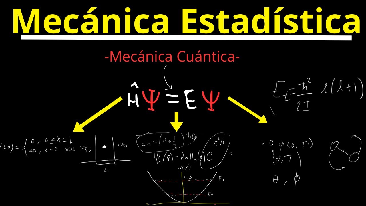
Let’s now return to the time-independent Schrodinger equation and see what else we can take from it. Recall that we have E times psi equals the kinetic energy operator acting on psi plus the potential energy operator acting on psi. But this sum of kinetic and potential energy operators is the Hamiltonian operator. This leads us to an interesting conclusion. The time-independent Schrodinger equation can also be written very simply like this, where the Hamiltonian operator acting on the wavefunction equals the eigenenergy of the particle times the wavefunction. What this means is that energy, E, is the eigenvalue of psi when the Hamiltonian operator acts on psi.
In this way, the Schrodinger equation is similar to some equations we have already learned.
We saw that when the position operator acts on psi, we get an eigenvalue of x. When the momentum operator acts on psi, we get an eigenvalue of p, which for a plane wave, will be equal to h bar k. And now, when the Hamiltonian operator acts on psi, the eigenvalue is E, which is the total energy associated with that wavefunction.
So again, it is this energy that, according to this equation, will determine the time-evolution of the system. That is, if you know the eigenenergy of a quantum state, and you know its wavefunction, you also know how it will evolve over time, and you can make actual predictions about it, just like the way you can predict the time-evolution of the classical motion of a particle. The only difference is that now you have to deal with uncertainty relations which are not a factor for macroscopic objects. And with that, we should have a better understanding of the Schrodinger equation in all of its forms, as well as precisely what these forms represent, and what we can do with them.
Up Next
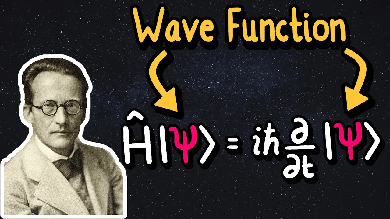
What a Quantum Wave Function Really Represents | Quantum Mechanics Basics
@ParthGChannel
29.5K views•2022-06-21

21cm Hyperfine Transition in Neutral Hydrogen: Radio Astronomy Basics
@AaronRobertParsons
12.4K views•2011-10-13

Radioactive Half-Life Practice Problem: Decay Constant & Fraction Remaining
@ProfessorDaveExplains
70.5K views•2019-10-29

Entropy and the Second Law of Thermodynamics Explained
@veritasium
27.5M views•2023-07-01
Related Study Plans & Knowledge Roadmaps
Structured learning paths in Physics