











![Shell and Tube Heat Exchanger Design - Kern's method [with sensitivity study] [FREE Excel Add In]](https://i.ytimg.com/vi/hZfu65IqcAg/maxresdefault.jpg)











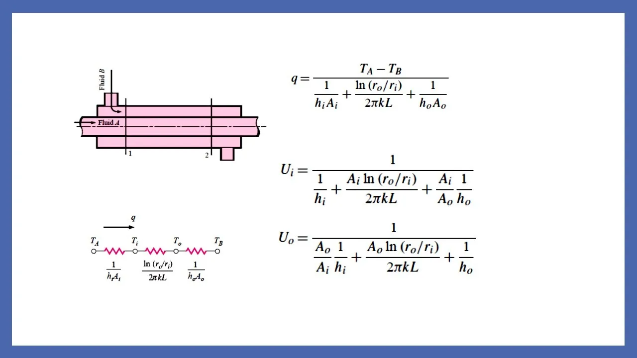
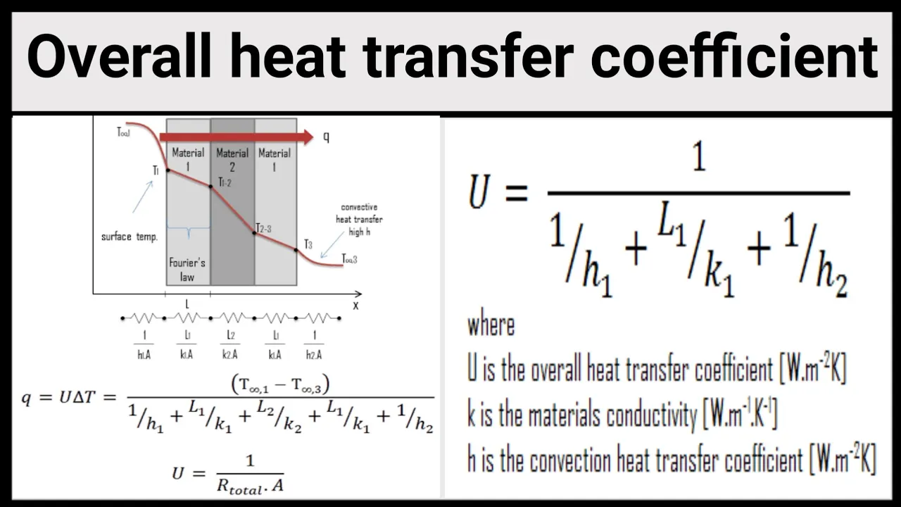
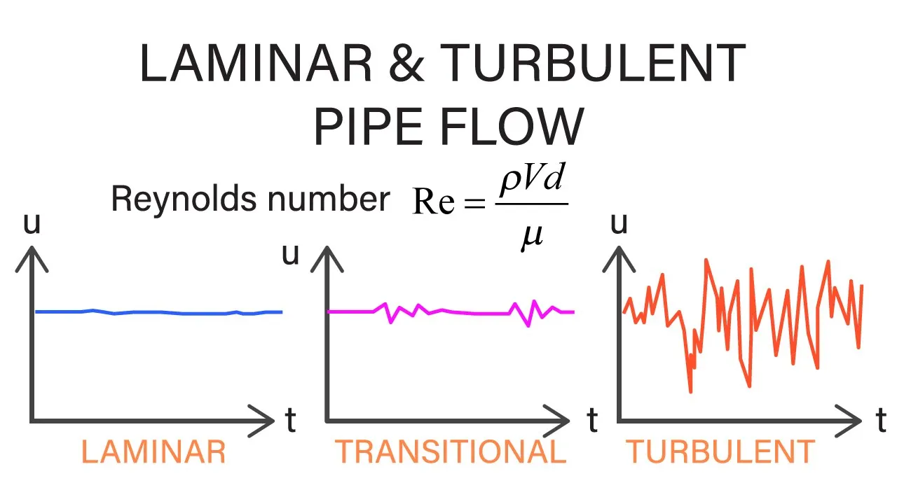
Heat exchanger design involves calculating the required heat transfer area using the formula A = Q̇/(U × ΔT_lm), where Q̇ is the heat transfer rate, U is the overall heat transfer coefficient accounting for convective resistances on both sides and conductive resistance through the wall, and ΔT_lm is the log mean temperature difference; pressure drop is estimated using ΔP = f × (L/D_H) × (ρV²)/2, where f is the friction factor dependent on Reynolds number and flow regime, L is the length, D_H is the hydraulic diameter, ρ is the fluid density, and V is the velocity, with the friction factor being 64/Re for laminar flow and approximately 0.2/Re^0.2 for turbulent flow.
Heat Exchanger Design: Area & Pressure Drop Estimation
Added:Fundamental principles of heat transfer, specifically conduction, convection, and the concept of the overall heat transfer coefficient (U).
Basic fluid mechanics, including fluid flow regimes (laminar vs. turbulent), Reynolds number, and pressure drop concepts in pipes.
Classical thermodynamics, specifically the first and second laws, entropy, and the fundamental concept of exergy (availability).
Standard heat exchanger analysis methods, such as the Log Mean Temperature Difference (LMTD) and Effectiveness-NTU (Number of Transfer Units) methods.
Detailed thermal design methodologies for specific industrial equipment, such as Kern's method or the Bell-Delaware method for shell-and-tube heat exchangers.
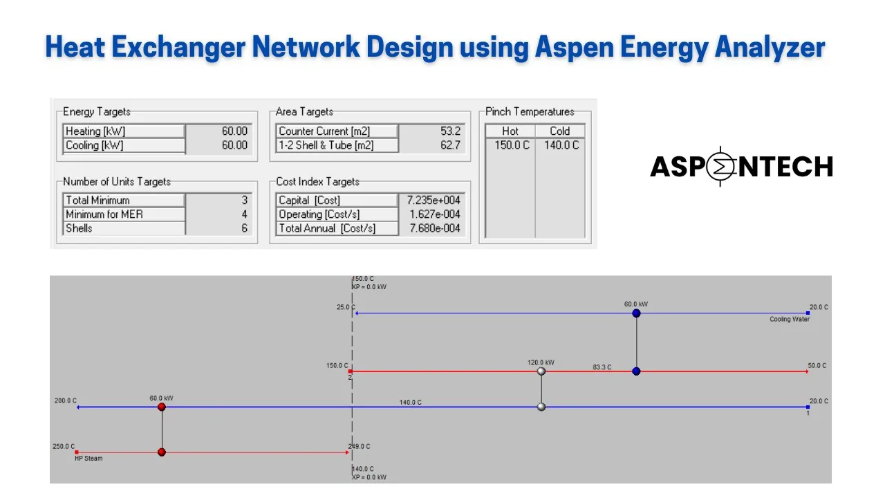
Pinch Analysis and Process Integration to optimize heat exchanger networks (HEN) within large chemical plants.
Dynamic simulation and control of heat exchangers under transient operating conditions using software like Aspen EDR or HTRI.
Study of advanced heat exchanger technologies, including compact, plate-fin, and microchannel heat exchangers for specialized applications.
Mechanical design standards (e.g., ASME Section VIII, TEMA standards) and addressing practical issues like fouling, vibration, and material corrosion.
112.7K views646likes37:55Original Release: 2014-02-22
hi and welcome to lecture number five in advanced power plant design then the spring 2014 semester Nick Seifert and in this lecture we're going to be looking at heat exchanger design and by the end we're going to be looking at we're going beginning to how you calculate both the area of the heat exchanger and estimating the pressure drop in a heat exchanger I just want to point out that our rule heat exchangers are really really complicated and you eat there's multiple by-path they could be by path so it could be in shell and tube heat exchangers you have flow going around bends there's you tube straight tube heat exchangers so one point out is the real world he exchanges extremely complicated and you probably need to be an expert to actually design one of these but in this course we're going to Adam simplifying these so that we can actually get it at least some estimates on the areas and then when we later in the course when we look at economics we're going to be using relationships between the area of a heat exchanger and its cost to estimate its cost one thing we can always do is we can always do a first line energy balance if you're a heat exchanger it's quite simple once you put your dashed line and you create your control volume the first law of thermodynamics is easy to state set the summation of the enthalpy entering the heat exchanger is going to be equal to and the summation of the enthalpy exiting the heat exchanger that's the case for an adiabatic when you make the approximation that we will be doing in this course at the heat exchangers adiabatic meaning heat is transferred from the hot side to the cold side but at no point time does any of that energy get transferred to the environment and we're also assuming that these heat exchangers there's no generation of work and that they're steady-state so when you make those approximations you get the equation shown in the bottom left of the slide so there's two main type of heat exchangers as far as which direction flow goes you can also have the third type which will be even more complicated where the flows are perpendicular but here we're going to take two simple cases one is Co flow in which the flow is actually the flow is going in the same direction so what happens is in a co flow at the very very beginning there's a huge temperature gradient and by the time you get to the exit you get to your smallest temperature gradient between the hot and cold side we we will probably never use Co flow heat exchangers in this course so I'm going to move now on to the counter flow and we'll be spending a lot more time with the counter flow in the counter flow the flows are flowing in opposite direction so what happens is that there is a temperature gradient on one side and there's a and then throughout the heat exchanger there's there's a temperature gradient and you can see in a counter flow case the gradient of the temperature difference between the hot and the cold side stays normally fairly constant it's very different than the co flow case in which there was very large difference between between one side and the other side and when you were trying to minimize extra tea destruction you want to have a small and constant heat exchanger delta T rather than if you and that's what you can get in the code it in the counter flow case and the co flow you have you end up having a region where there's a lot of extra G just structure at the front and then by the time you get to the end you one thing to notice is that the temperature gradient gets small and here's the key thing why we typically don't use Coco flow is that in the co flow the outlet temperature on the cold side is limited by the outlet temperature on the hot side which means that you can never get that temperature above the temperature of the outlet of the hot side whereas in the counter flow case you can get your temperature on the outlet of the cold side to be above the temperature of the outlet on the hot side you're only constrained in that case by the temp actual temperature on the inlet of the hot side and that's going to be key this this would be a particularly case um and something we won't cover with a solid oxide fuel cells you may have a temperature difference between the hot cold side of let's say 50 degrees right but the overall temperature increase from the cold Inlet to cold outlet maybe up to 500 degrees Celsius and from the safe room temperature to 500 so to 500 degrees C and that's only going to be possible if you're in a counterflow design so here's what a general tower flow heat exchanger would look like okay in which this is a case in which the temp there's a temperature change across the heat exchanger the driving force changes with across the heat exchanger so we've got the inlet and the outlet and as I mentioned before that temperature cold on the outlet can be above the temperature on the outlet of the hot side and so we're going to use the symbol delta T sub y is the driving force for heat transfer and that changes across from Y is equal to 0 to Y is equal to Y we're here on the on the x-axis is the distance along the heat exchanger Y and on the y axis we're graphing the temperature so I want to point out that an extra G analysis is fairly easy to do for a heat exchanger and for a steady-state system when there is no heat being transferred to the environment this breaks this can be simple in assuming steady state we can calculate the extra G destruction as basically just the summation of the Inlet extra G's minus the outlet extra G's and so this is what the EDD equation looks like and now I want to point out just so we can build some intuition I'm going to actually we're going to solve for the extra G destruction for in the heat exchanger under one simple case just to help build some intuition on how the XUV destruction depends on some of the variables so what we're going to do here is we're going to have a couple variables we have the temperature cold side Inlet okay let me um step back a second we're going to solve this under a particular case in which the flow rate on the hot side multiplied by the CCP on the hot side is equal to the flow rate on the cold side multiplied by the CCP on the cold side and under that case what you get is that the temperature difference between the hot and cold side is a constant across the heat exchanger and that greatly simplifies the calculations so that that temperature gradient we're calling delta T 1 and what we're calling delta T 2 is the actual temperature rise from any of the inlet from the inlet to the outlet or vice versa on the hot side from the inlet to the outlet and under this particular case where n dot times C sub P is equal to constant you can find that the extra G destruction I or the irreversible entropy destruction times the temperature of the environment okay so the Sigma dot irreversible is going to be linearly proportional to the N dot which should make sense right more x2 destruction for a larger when you have more flow and CCP it also increases with CCP right it which means more heat is being transferred and what I want to point out here is when you solve that equation you get n dot times CCP times the logarithm and inside the logarithm is one plus delta T 1 times delta T 2 divided by the temperature on the cold side Inlet multiple divided by the temperature on the hot side Inlet which is TC inlet plus delta T 1 plus delta T 2 so the key thing to note here is that when the temperature on the cold side Inlet goes to infinity what you find is that there is no entropy irreversible entropy generation which means if you have something really hot transferring to something else that's also fairly hot then there is no extra G destruction right which would make sense from a cart from a Carnot efficiency point of view if your temperature is 6,000 you're transferring it down to something at 5,000 degrees there's virtually no exergy destruction okay so that's one that's the easy thing to point out next thing I point out is so let's say the temperature cold on the inlet is closer to room temperature the exergy destruction increases with delta T 1 meaning the greater the driving force the greater the extra G destruction and it's also going to increase with delta T 2 where delta T 2 is can be seen as the total amount of energy transferred so in the case where the what's inside the logarithm the 1 plus term over here when when that term on the right is small right a logarithm of 1 plus a small number is close to that small number so logarithm of the quantity 1 plus X is roughly X so in that case what you find is that the extra G destruction Sigma dot irreversible times which is Sigma dot irreversible times T naught would be equal to T naught times n n dot times C CP times delta T 2 times delta T 1 and divided by temperature cold on the inlet I'm sensor hot inlet and so what you can see here is extra destruction is going to go up notice that a amount of heat transferred would be equal to n dot times C CP times delta T 2 right so extra G destruction is going to be equal to that the amount of heat transferred times the gradient and then divided by some of the temperatures on the inlet side so more exergy destruction occurs when there is a greater driving force when more heat is transferred and it decreases as the is you increase the temperature of the entire system like the cold on the cold side so that's way I just want to build some intuition here the one thing the main thing I want to get out of this is that the larger the driving force the more the extra t destruction okay so now we're going to move on to how do we actually estimate the area of a heat exchanger and then from that the other question we're going to need is not only area but we're going to need to know the pressure drop through a exchanger so the area of it using fully errors law we can estimate that the area is going to be equal to the amount of heat transferred divided by the log mean temperature difference and then we're going to be multiplying that by the quantity one over the heat transfer coefficient on the cold side plus the thickness of the metal that is separating the hot side from the cold side divided by the thermal conductivity of that metal plus one over the heat transfer coefficient on the hot side that's H sub H in this case here so what one you'd imagine is that there are three resistors in series and that so just like in the electrical resistor case you had a voltage three resistors and then ground so in this case ground is can be thought of as the temperature on the cold side the voltage is the temperature in the hot side and we have three resistors we have the resistance for heat to flow from the temperature in the center of the hot side of the heat exchanger to the wall separating the hot from the cold side right he has to transfer from the if this is a gas or gas or liquid it's got if it's got to transfer from the center to the wall it's got to go through the wall so that's the resistor number two and then from the wall it's got to transfer to the cold side gas or liquid so that's what we have here is we have three resistors in series so we're basically figuring out that the area is going to go is going to increase of course as you increase the resistance of all each of those resistors the easy one to think about is the one in the middle the the metal is this if it's a metal like steel which is used a lot as steel or aluminum and heat exchangers the as you could increase the distance or the thickness of the wall material separating the hot from the cold side you can be ended up and end up increasing the resistance and hence increasing the area of the heat exchanger so before we go on to learn more about how we calculate the H sub C and H sub H I want to point out that on I want to give the definition of the log mean temperature difference and that definition is that the log mean temperature difference is the difference between the hot and cold side at y is equal to zero minus the temperature difference between the hot and cold side at y is equal to l so those are the two ends of the heat exchanger and then we're going to be dividing that by the logarithm of those two differences of the logarithm of the ratio of those two differences when the differences are equal you'll notice that this equation looks like is zero divided by zero so you have to use a layup l'hospital's rule and what you'll find is that the logging temperature is just equal to th minus TC which is a constant in this case as you would expect and so want to point out a couple assumptions that kind of go into the first equation the these equations are valid if the thermal conductivity is not of the wall or of the material itself of the gas or liquid is not a strong function of temperature and if the specific heat of the fluid is not a function of temperature these are not true in general but still this equation is a can be fairly safe to use when you're not talking about major increases in temperature across the material in that case you might need to do a more realistic model that um but for the estimate we're using this eventually in cost estimating this equation is extremely useful and we'll be using it in this course because of its usefulness because if not you would actually have to integrate along the length of the heat exchanger to figure out the area required so one of the assumptions I mentioned was that the thermal connectivity is not a strong function of temperature so what I've graphed here is I want to point out the thermal conductivity can be is definitely a function of temperature and I'm graphing here the thermal conductivity of stainless steel when you're at low temperatures the conductivity is a huge function of temperature but once you get to 300 degrees Kelvin I've shown here 300 degrees Kelvin the conductivity is about 140 milliwatts per centimeter Kelvin whereas when you get out to 500 Kelvin it's only about 170 milliwatts per centimeter Kelvin so it is a function of temperature but you can fairly safely just take the average value and and the equation above will be valid so take the average so when you're using connectivity's use the average value between the temperatures on the on the heat exchanger when opponent gives some values that you can use it point out that aluminum has a very very high thermal connectivity which is nice because it means that you can keep down on the area the heat exchangers as the value about 215 watts per meter Kelvin carbon steels have a decent value of thermal connectivity if you need Steel's that can handle maybe fluids that might be caustic so sodium hydroxide in aqueous solutions you're likely going to need stainless steels or stainless steel 316 and you can see here that their thermal conductivities decrease so and and that is a somewhat unfortunate thing because what it means is that as you as you make the steel more tolerant to impurities and to caustic materials it's heat transfer coefficient drops which is one not only also compared to carbon steel stainless steels are more expensive so this is one of the things that um you have to watch out for when you design power plants is that you can't just say you design something for carbon steel and the two is kind of a flue gas going to a ranking site you know heating up the water on a ranking cycle if you just were to swap out into a stainless steel not only to your costs increase just because of the material but you also have to look at the fact that your heat transfer coefficient is likely dropped significantly and that could have a negative effect on their overall powerplant so if you meant in the equation there were the heat Cove heat transfer coefficients those H's so on point what a one point out here is that H is a function of the Reynolds number of the flow and when you're in the laminar flow H has a fairly simple equation which so laminar here being that a Reynolds number is less than about 2000 in that case heat transfer coefficient is approximately four times the thermal conductivity of the fluid divided by the hydraulic diameter D sub H G sub H is the hydraulic diameter and it's a hydraulic diameter is a ratio of the perimeter in area of a tube so this what we see here is it's a constant times the thermal conductivity divided by the hydraulic diameter when you get to turbulent flow so that was a foot laminar case when you get determine your flow which is roughly Reynolds number greater than five thousand the equation is a lot more complicated now H is not only a function of K over D of the hydraulic thermal conductivity of the fluid divided by the hydraulic diameter is is now a function of the Reynolds number and the prandtl number of the fluid the rent the Reynolds number is the hydraulic diameter times the velocity divided by the kinematic viscosity so it this can also be put it be put in terms of the dynamic viscosity and that is such that you have the mass density times the hydraulic diameter times the velocity divided by the dynamic viscosity so that's the Reynolds number low low Reynolds number is lammer high Reynolds numbers is turbulent well part the Prandtl number is a ratio of the kinematic viscosity to the thumb to the thermal connectivity here when you put in in units that were more used to it's the specific key constant of the fluid times the fluid dynamic viscosity divided by the thermal conductivity the here's I just want to point this out again if you take the heat transfer coefficient times the hydraulic diameter and divided by the thermal conductivity you have something called the new tilt number and so the neutral number is equal to roughly 4 when you're in the laminar region and then you can see it increases and once you get into turbulent flow that's the neutral numbers now goes like the Reynolds number to the point eight power so this is a graph and I'm showing the website below where you can access the where where this graph comes from it's from a heat transfer textbook and the data is actually in that book is actually from a paper by Chris and it's using data from air in in a heat transfer pipe so this is actual data on from air as looking at the basics of the heat transfer coefficient as a function of the Reynolds number so of course we want to be able to estimate the viscosity of a gas because we're going to be needing to know that when we design heat exchangers so there is luckily a fairly simple equation for the viscosity of a gas itself as opposed to the viscosity of liquids can be extraordinarily complicated the viscosity of liquids is pretty simple and so the equation in in variable form is that the dynamic viscosity of a gas is equal to the mass density times the velocity times the mean free path of collisions divided by three and for gases you can solve that this is roughly equal to two point seven times ten to the minus six times the square root of the the molar mass of the gas times the temperature that's all in the square root and then divided by the cross-sectional area squared times Sigma sub u Sigma sub Nia where Sigma sub u sub mu is a cross-sectional integral Oracle oh sorry a collision integral and it's defined at the very bottom here big Sigma Sigma sub mu is a roughly equal to 1/2 plus one point 1 divided by X to the zero point six we're here X is equal to the actual temperature divided by epsilon epsilon here is the lennard-jones well depth we talked before about grandeur wall gases if you remember in van der Waal gas we had that well depth well here the well depth for Leonard Joan is very very similar same kind of concept we have some kind of well depth and in lennard-jones there's also the size which was size went kind of like that B coefficient and the depth kind of went like a and a vandals van der Waal gas so here that well depth is given in units of Kelvin and it it's a depth it's like an energy depth and you're basically dividing it by the Boltzmann constant to be able to turn that into an epsilon into a temperature and so you can see here that well depth is particularly large for water vapor and it's really small for hydrogen okay so when you have that clue when you have those when you have that the well depth D that goes into the Sigma sub mu and the lennard-jones size which goes into the collision cross-section you can now calculate the viscosity of a gas I want to point out the thermal conductivity of a gas is also fairly easy to calculate once you have the viscosity you just multiply it by the quantity C sub P plus one point two five times R so it'd mean if you know the specific heat constant and you know the viscosity then you know the thermal connectivity of a gas and so in the on the slide before we said that the parental number look like C sub P times mu divided by the thermal connectivity so if there was a relationship so for for gases since there's a there's a relationship between K mu and C sub P what we find is that the Prandtl number of a gas is equal to four times gamma divided by the quantity nine gamma minus five so gamma being the ratio of specific heats C sub P which is C sub P divided by C sub V once you know that for a gas then you can very quickly calculate the Prandtl number and then for error it's a value of about 0.7 so the last thing we're going to be doing this lecture is looking at the pressure drop and we're going to be needing to know the pressure drop because if we were to make the heat exchanger larger and larger larger we would find that the pressure drop would continue to increase if we make the length of the heat exchanger longer and longer we find that the pressure drop would increase and we have to somehow pay for this your job pressure drops you know don't come from for free it typically means that you have some compressor you're gonna have to run hard more power and hence less power from your power plant so when we get to the optimization part of this course later on we need to know both the area of the heat exchanger so we can estimate the cost but we also need to know the Delta P because we need to know how much compression we're going to want to need to supply to overcome that Delta P so let's go through quickly how we estimate the pressure drop so the pressure drop is going to be equal to the friction factor times the length divided by the hydraulic diameter multiplied by the mass density times the velocity squared over two so the rate of thing about this is that pressure drop increases with friction increases with length increases with velocity and is going to decrease as you increase the hydraulic diameter so there's other ways of writing this equation you can see here you can put it in terms of the Reynolds number because you maybe don't know the velocity but you know the Reynolds number and or what if the last of these equations put the pressure drop is equal to the friction factor multiplied by the molar mass multiplied by the float the molar flow flow velocity well is in moles per second that's squared multiplied by the length divided by two times the molar density times the number of tubes squared times the hydraulic diameter to the fifth so let's think about this for a second so as the friction increases right we got more of a pressure drop as we try to put or flow through the system it's going to go like the pressure jobs can go like the flow squared it's going to also go increase with the length literally with the length it's going to be inversely proportional to the molar density so when you have something that's very very dense you're going to be having less pressure drop than for something that is not dense for if you have the same amount of moles per second going through building I want to point out is you this the pressure drop goes like the number of tubes to the minus 2 power right more the more tubes you have the less pressure drop now the more tubes you have probably going to be more costly right as far as capital costs so you can see that there's likely going to be some kind of optimal number of tubes where if you don't have enough tubes you can have a huge pressure drop and you got to pay for that in compressor but if you have too many tubes you're going to end up paying for it Inc up in capital costs and the same is true for the hydraulic diameter you can see here goes as the inverse lead to the two egos as the minus 5 power so once again there's going to some kind of optimal hydraulic diameter to these tubes and that's what we'll get into later in this course is how do we actually solve for with that optimal number of tubes is and diameter of the tubes the next thing I want to point out is how did the friction factor is defined both in the laminar and turbulent regimes and in the laminar regime the friction factor looks like 64 of the Reynolds number so if you know you're in the laminar regime it's a really simple equation if you know you're in the turbulent regime like greater than 5,000 friction factor it looks like 0.2 divided by the reynolds number to the point 2 plus about 0.01 8 that's if you have a tube whose roughness factor epsilon is equal to zero point zero zero one so I want to point out that equation is only valid when the the roughness thickness divided by the diameter of the tube hydraulic diameter of the tube is equal to about is equal to point one percent but that is that I use that value because that is a very typical value of epsilon for us for steel pipes when you read between 2,000 and 5,000 Reynolds numbers you need to use some kind of approximation and you can roughly approximate that the friction factor looks like a combination from the laminar and turbulent regimes and so that combined equation can is roughly valid over the entire span of of course when you're it when you know you're in the laminar you should be using just the laminar equation so what I want to point out here is so you can solve for the area but we know that there's a relationship between the area and the length L so you can solve for the pressure drop when you solve for the length using the a is equal to Q dot / LM TD equation solve for the length and put that into the equation for the pressure drop and then if you make an approximation to if you assume something have an isothermal compressor you can make an approximation to how much work is consumed to overcome that pressure drop and you now have an equation that shows how the work is going to increase with the flow rate cubed right so more flow you have you're going to require a lot more work the delta T is getting the work required to overcome the pressure drop goes like the Delta increases linearly with the amount of heat that needs to be transferred to heat up the fluid it's going to go like the number of tubes to the minus 2 power alright so the more tubes you have the less work it's going to go like the hydraulic diameter to the minus 4 power so that means the larger the tubes the less work you need it's going to go like the log mean temperature difference inversely so this is one thing I want to point out here the amount of work needed to make up for the Delta P this is a frictional loss of work goes inversely with the log mean temperature difference so you'd think well let's have a log mean temperature difference but of course the exergy destruction in the heat exchanger due to heat transfer is going to be linear with the log roughly linear to the log mean temperature difference so you can see once again there's going to be some kind of optimal value of the log mean temperature difference because you can see the overall amount of extra to destruction looks like it's going to have some term divided by log mean temperature difference plus some other constant multiplied by log mean temperature difference in and basically optimization of X plus 1 over X you find that there's going to be an optimal value there's going to be some point in some optimal log mean temperature difference just as there's going to be some optimal number of tubes and hydraulic diameter but to really do this we're going to of course need to introduce economics which we won't be covering for quite a number of lectures but I just want to hopefully build your intuition about what's going on here with heat exchangers how we calculate the area and how we calculate the pressure drop so we can try to figure out how expensive the heat exchanger is going to be and how much work is going to be required to overcome the pressure difference you
Up Next

33:40
CPU Water Block Comparison: Alphacool Core 1 vs. EK Magnitude
@der8auer-en
126.3K views•2023-08-20

30:32
Ultrasonic Transducers: Resonant Frequency Measurement and Horn Design
@imajeenyus42
229.9K views•2017-02-22

54:16
Polymer Environmental Degradation: Mechanisms & Stabilization
@iit
1.8K views•2012-07-10

33:39
How a Student's Question Saved a NYC Skyscraper from Collapse
@veritasium
22.8M views•2025-04-26
Related Study Plans & Knowledge Roadmaps
Structured learning paths in Engineering
engineering
Building Acoustic Levitators: Physics & Arduino
01The Physics of Sound and Standing Waves
02Piezoelectric Transducers and H-Bridge Drivers
03Arduino Programming: Generating 40 kHz Signals
+ 2 more learning modules
14h5 modules
Explore Roadmap
engineering
Building Peltier Cloud Chambers: Particle Tracks
01Cosmic Rays & Cloud Chamber Physics
02Thermoelectric Cooling (TEC) Fundamentals
03Custom Liquid-Cooling Loop Design
+ 2 more learning modules
18h5 modules
Explore Roadmap
engineering
Yagi-Uda Antennas: Modeling, Build & VNA Test
01Introduction to RF and Antenna Fundamentals
02Yagi-Uda Antenna Design Principles
03Antenna Modeling and Simulation in 4NEC2
+ 2 more learning modules
18h5 modules
Explore Roadmap
engineering
ECG Monitor Design: Op-Amps, Filters & Noise
01Electronics & Breadboard Basics
02Op-Amps and Instrumentation Amplifiers
03Bioelectricity and ECG Fundamentals
+ 2 more learning modules
18h5 modules
Explore Roadmap