

















Surface urban heat islands occur when impervious urban surfaces like asphalt and concrete absorb and retain more solar heat than natural landscapes, creating elevated temperatures in urban cores relative to surrounding rural areas; these can be mapped using satellite thermal infrared sensors such as Landsat 8/9 and MODIS, with intensity calculated as the temperature difference between urban and rural areas, and analyzed through platforms like Google Earth Engine to support urban planning and public health interventions.
NASA ARSET: Mapping Urban Heat Islands with Landsat & MODIS
Added:Basic principles of remote sensing, including the electromagnetic spectrum and how thermal infrared sensors detect heat radiation.
The conceptual distinction between Land Surface Temperature (LST) and ambient air temperature.
Fundamentals of Geographic Information Systems (GIS) and working with raster data formats.
An introductory understanding of the Landsat and MODIS satellite missions, including their spatial and temporal resolution differences.
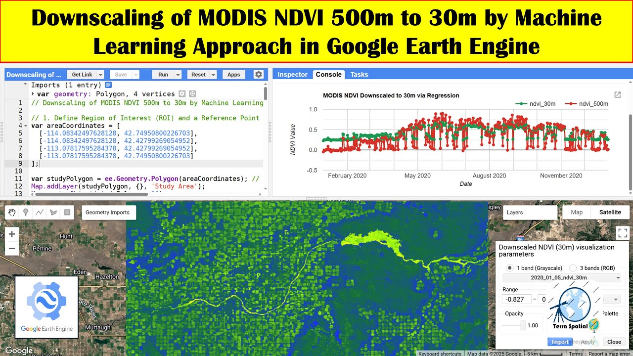
Advanced data fusion and downscaling techniques to combine the high spatial resolution of Landsat with the high temporal resolution of MODIS.
Application of urban heat island mapping to urban planning, climate adaptation policies, and green infrastructure design.
Integration of LST data with socioeconomic and demographic datasets to perform thermal vulnerability and environmental justice assessments.
Utilizing microclimate modeling software (such as ENVI-met) to simulate the cooling efficacy of local-scale urban interventions.
18.1K views360likes1:02:44Original Release: 2022-08-04
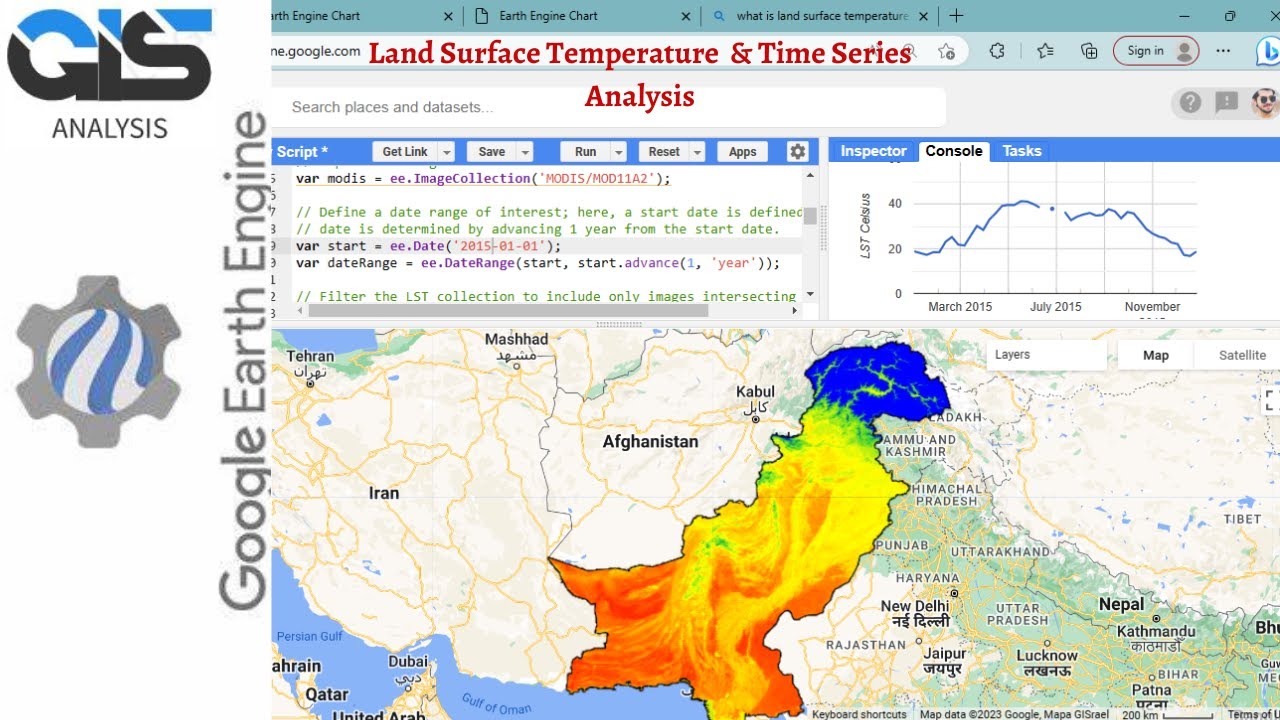
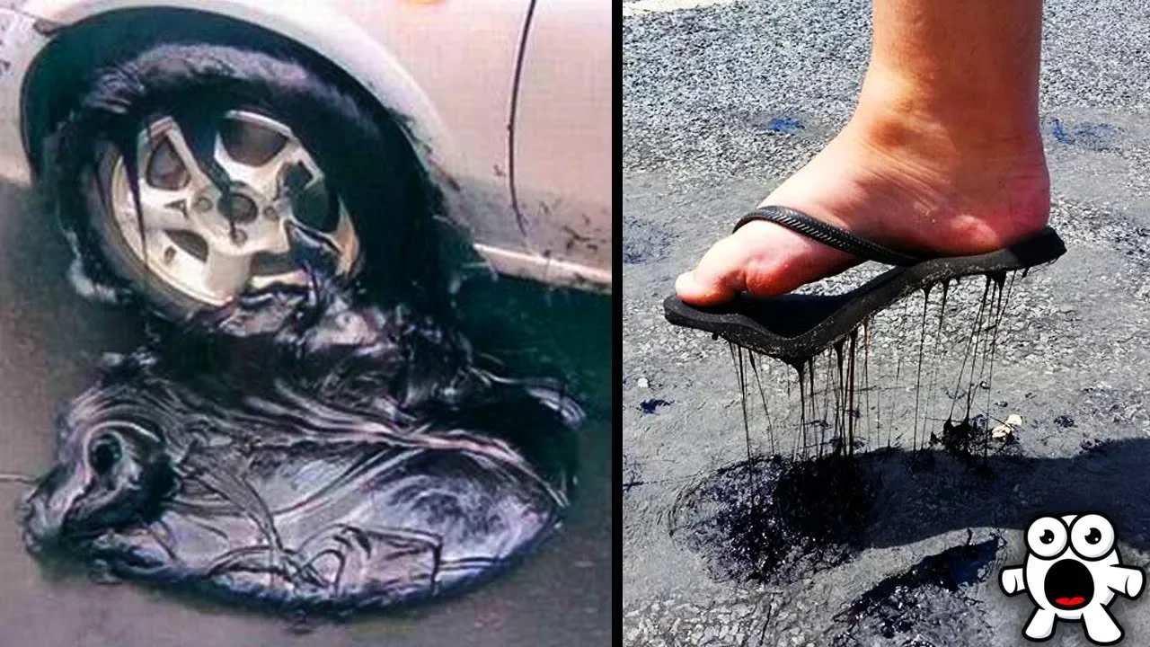
welcome to part one of the rset training satellite remote sensing for measuring urban heat islands and constructing heat vulnerability indices my name is sean mccartney and i'm an arset trainer from nasa's goddard space flight center in this first part of the webinar series i'll be presenting and demonstrating methods for land surface temperature based urban heat island mapping this training is an advanced four-part webinar series covering topics ranging from land surface temperature mapping of urban heat islands to integrating socioeconomic data with satellite imagery for constructing heat vulnerability indices the final part of the training will present how to use high-resolution satellite-derived heat estimates and gridded population data to map extreme heat exposure worldwide there will be hands-on exercises in parts one and three for you to work with satellite imagery and learn how to construct your own heat vulnerability indices each of the four parts of the training will be one and a half hours in duration including presentations lab time in parts one and 3 and question and answer sessions the same content will be presented at two different times each day please only sign up for and attend one session per day all webinar recordings presentation materials code and homework assignment can be accessed from the training page provided at the link below there will be one homework assignment for this webinar series comprising questions from all four parts of the training be sure to follow the instructions carefully as some questions will involve submitting screenshots of the results from the hands-on exercises answers must be submitted via instructions found on the training page the due date for the homework assignment is august 25th a certificate of completion will be awarded to those who attend all four live webinars and complete the homework assignment by the deadline you will receive a certificate approximately two months after the completion of the course from marines martin the following are prerequisites for today's training if you wish to use today's lab time and work with the javascript code we're providing to calculate urban heat islands you'll need to register an account with google earth engine once you've registered an account using a gmail or edu email you'll have access to the shared repository accessing the scripts from the training the other prerequisites are the fundamentals of remote sensing course and the satellite remote sensing for urban heat island scores presented by rset in 2020 the first training provided more theoretical background on urban heat island while today's training is meant as a refresher while giving participants more time to work with the code and analyze satellite imagery for assessing urban heat islands in your own area of interest after participating in today's training attendees will be able to define what an urban heat island is and why it matters to urban planners and public health experts identify which satellites and sensors can be used for assessing urban heat islands analyze land surface temperature from landsat 8 and 9 and aqua modis using google earth engine and summarize the limitations of satellite data for understanding urban heat islands for those unfamiliar with the applied remote sensing training program or rsat rsat is part of nasa's applied sciences capacity building program rcit provides accessible relevant and cost-free training on remote sensing satellites sensors methods tools and applications trainings are offered online and in person for beginners and advanced practitioners alike trainings cover a range of data sets and tools and their application to air quality agriculture disasters land and water resources management our set's goal is to increase the use of earth science remote sensing and model data in decision making through training for professionals in the public and private sector environmental managers and policy makers trainings are freely available to anyone with an internet connection and conducted either live instructor-led or self-guided such as our fundamentals to remote sensing since 2009 the program has reached over 50 000 participants from over 170 countries all rsap materials are freely available to use and adapt for your curriculum if you use the methods and data presented in rc trainings please acknowledge the nasa applied remote sensing training program i'll now present an overview on urban heat islands before delving into the applications of satellite remote sensing to monitor this phenomenon structures such as buildings roads and other infrastructure absorb and re-emit the sun's heat more than natural landscapes such as forests and water bodies urban areas where these structures are highly concentrated and greenery is limited become islands of higher temperatures relative to outlying areas these pockets of heat are referred to as heat islands differences in temperature has to do with changes in radiative and thermal properties of impervious surfaces heat islands form as vegetation is replaced by asphalt and concrete for roads buildings and other structures necessary to accommodate growing populations these surfaces absorb rather than reflect the sun's heat causing surface temperatures and overall ambient temperature to rise displacing trees and vegetation minimizes the natural cooling effects of shading and evaporation of water from soil and leaves there are different causes for the urban heat island phenomenon surface albedo is a measurement of the reflectivity of solar energy on earth's surface the measurement varies from 0 to 1 where a value of 0 characterizes a surface that absorbs all incoming energy and a value of one characterizes a surface that reflects all incoming energy asphalt concrete and brick have very low albedos meaning they absorb rather than reflect the sun's heat causing surface temperatures and air temperatures to rise due to their thermal storage capacity often heat islands build throughout the day and become more pronounced after sunset due to the slow release of heat from asphalt concrete and brick trees vegetation and water bodies tend to cool the air by providing shade transpiring water from plant leaves and evaporating surface water when we reduce vegetation in urban areas there is less shade and moisture than natural landscapes which contributes to higher temperatures vehicles air conditioning units buildings and industrial facilities all emit heat into the urban environment these sources of anthropogenic waste heat contribute to heat island effects the dimensions and spacing of buildings within a city influence wind flow and urban materials ability to absorb and release solar energy in heavily developed areas surfaces and structures obstructed by neighboring buildings become large thermal masses that cannot release their heat readily calm and clear weather conditions result in more severe heat islands by maximizing the amount of solar energy reaching urban surfaces and minimizing the amount of heat that can be carried away conversely strong winds and cloud cover suppress heat island formation geographic features can also impact the heat island effect large bodies of water can moderate temperature while nearby mountains can block wind or create wind patterns that pass through a city urban heat islands can form during the day or night in small or large cities and in any season of the year urban rural temperature differences are often largest during calm clear evenings this is because rural areas cool off faster at night than cities which retain much of the heat stored in roads buildings and other structures as a result the largest urban rural temperature difference or maximum heat island effect is often hours after sunset the diagram on the right of the slide shows the heat allen effect with the orange lines being the temperature in the day and the blue lines being the temperature at night parks open land and bodies of water create cooler areas within a city when we speak about the urban heat island effect it's good to recognize that there are two types of urban heat islands surface urban heat islands and atmospheric urban genomes surface urban heat islands form because urban surfaces absorb and emit heat to a greater extent than most natural surfaces and tend to be most intense during the day when the sun is shining atmospheric urban heat islands form as well as a result of warmer air in urban areas compared to cooler air in outlying areas atmospheric urban heat ions vary much less in intensity than surface heat islands surface urban heat islands represent the radiative temperature differences between impervious and natural surfaces and as previously mentioned tend to be the most intense during the day when the sun is shining the magnitude of surface urban heat islands varies with seasons but it's typically largest in the summer surface urban henons are primarily measured in the thermal infrared region of the electromagnetic spectrum and are normally observed with radiometers fixed to remote platforms these remote platforms can be satellites airplanes meteorological towers or building rooftops satellite thermal remote sensing has the advantage of offering global and seasonal coverage of surface heat islands and provides consistent and repeatable observations of the earth's surface satellites in particular are advantageous for observing surface heat islands at spatial scales ranging from neighborhoods to metropolitan regions and for enabling simultaneous and spatially continuous measurements of surface temperature across a hierarchy of scales when assessing surface urban heat ons using satellite imagery the intensity of the heat island can be characterized by the temperature difference between the average temperature of the urban core window and the average temperature of the rural window as seen in the equation on this slide this is the simplest quantitative indicator of the thermal modification imposed by urban areas relative to non-urban areas when we explore land surface temperature using satellite imagery we'll provide examples of deriving surface urban heat island intensity and how you can calculate this for your own area of interest so why are urban heat islands a problem higher daytime temperatures and reduced nighttime cooling contribute to heat related deaths and heat related illnesses heat islands can also exacerbate the impact of naturally occurring heat waves which many of us are currently experiencing this summer in the northern hemisphere children older adults and those with existing health conditions are particularly at risk populations with low income are at greater risk of heat related illnesses due to poor housing conditions including lack of air conditioning and small living spaces and inadequate resources to find alternative shelter during a heat wave heat islands increase both overall electricity demand as well as peak energy demand peak demand generally occurs on hot summer weekday afternoons when offices and homes are running air conditioning systems lights and appliances during extreme heat events which are exacerbated by heat islands the increased demand for air conditioning can overload systems and require utility to institute controlled rolling brownouts or blackouts to avoid power outages companies that supply electricity typically rely on fossil fuel power plants to meet much of the demand which in turn leads to an increase in air pollution and greenhouse gas emissions in addition to their impact on energy related emissions elevated temperatures can directly increase the rate of ground level ozone formation ground level ozone is formed when nitrogen oxides and volatile organic compounds react in the presence of sunlight and hot weather high temperatures of pavement and rooftop surfaces can heat up storm water runoff which drains into storm sewers and raises water temperatures and is released into streams rivers ponds and lakes water temperature affects all aspects of aquatic life especially the metabolism and reproduction of many aquatic species rapid temperature changes in aquatic ecosystems resulting from warm storm water runoff can be particularly stressful and even fatal to aquatic life we'll now pivot to focus on how remote sensing can be used to monitor urban heat islands as stated earlier urban hedons are primarily measured by remote sensing in the thermal infrared part of the electromagnetic spectrum when electromagnetic radiation travels through the atmosphere it may be absorbed or scattered by the constituent particles of the atmosphere between approximately 10 to 12 micrometers the atmosphere has relatively low absorption absorption of infrared radiation emitted by the land surface it is within this atmospheric window space foreign instruments observe the thermal infrared spectral region to derive land surface temperature the image on the right of the slide shows atmospheric windows where specific types of electromagnetic radiation can freely pass as well as absorption bands where the atmosphere absorbs and scatters electromagnetic radiation this slide shows the satellites sensors temporal coverage orbit and swath spectral bands spatial resolution and temporal resolution for each nasa mission we'll be covering in today's case study we're focusing on the landsat missions since the united states geological survey or usgs recently released the collection 2 archive this provides a surface temperature product so you no longer have to calculate land surface temperature from ancillary datasets such as emissivity and vegetation indices we're also focusing on the moda sensor since it has historic data going back two decades and provides both day and night surface temperature products usgs released landsat collection 2 in december 2020 and is the second major reprocessing effort on the landsat archive resulting in several data product improvements that applied advancements in data processing algorithm development and data access and distribution capabilities landsat collection 2 contains level 1 data from landsat 1 through 9 and science products from landsats 4 through 9 including scene-based global level 2 surface reflectance and a surface temperature science product collection 2 also provides improved radiometric accuracy improved radiometric calibration consistent quality assessment bands among other improvements landsat surface temperature measures the earth's surface temperature in kelvin and is an important geophysical parameter in global energy balance studies and hydrologic modeling surface temperature data are also useful for monitoring crop and vegetation health and extreme heat events such as natural disasters and urban heat island effects the second land surface temperature product we'll be demonstrating in the case study is modis surface temperature from the aqua satellite it is also based on thermal infrared bands and comes with a one kilometer spatial resolution the modis land surface temperature product derived from the aqua mission contains surface temperature for both day and night historical data runs from 2002 until present in both daily and eight day average temporal height latency below are some of the benefits of using satellite remote sensing for urban heat islands satellites provide continuous spatial coverage compared to in-situ data they provide data where no systematic in-situ measurements are available and they augment where in-situ measurements currently are they provide simultaneous observations of land surface temperature surface emissivity and land cover from various satellites satellites provide global timely consistent data coverage and thanks to nasa and other space agencies open source policies availability of data is freely and publicly available to anybody on the planet below are listed some of the limitations of satellite remote sensing for urban heat islands data acquisition times of sun synchronous satellites usually do not coincide with the time of day where the surface urban heat ion is at a minimum or maximum landsat only provides daytime data not nighttime data optical sensors cannot penetrate clouds or vegetative cover which can lead to data gaps or a decrease in data utility the accuracy land surface temperature estimates depends strongly on corrections for atmospheric effects and on accurate estimate of surface emissivity radiate radiate instances received by sensors are influenced by the sensor viewing angle it is difficult to obtain high spectral spatial and temporal resolution with the same instrument and a large amount of data exists in various spatial and temporal resolutions file formats sizes and from multiple sources now that we've had a refresher on urban heat islands and a background on specific satellite missions used to observe urban heat islands we'll discuss how to use google earth engine to access analyze and visualize land surface temperature from landsat and modis google earth engine is a cloud-based geospatial analysis platform that combines a multi-petabyte catalog of satellite imagery and geospatial datasets with planetary scale analysis capabilities enabling users to visualize and analyze satellite images of the planet the platform comes with a javascript editor though python is available as well it is free to register an account using a gmail or a.edu email address to browse the catalog of satellite imagery and geospatial datasets as well as signing up for a free account refer to the links below for resources resources to learn more about google earth engine refer to the links to the developer's guide and the developers group provided on the slide we're providing you with three scripts of example code to analyze land surface temperature and the surface urban heat on effect using google earth engine the production chain was fully coded in javascript using the code editor platform scripts are freely available using the links below all input data sets to the land surface temperature algorithm are obtained from the google earth engine data catalog once you've registered an account with google with earth engine you'll be able to launch the application using the links provided on the slide the first script shows how to graph a land surface temperature time series from landsat 8 and 9 for any user specified longitude and latitude the second script shows how to process landsat derived surface urban heat island over washington dc but can be adapted for any other city on the planet the third script shows how to process modis derived surface urban heat on for both day and night over washington dc but can also be adapted to any other city on the planet the code for the three separate skips has been commented commented throughout explain explaining which parameters need to be changed for your own area of interest and on this slide we're providing the main parameters you'll need to modify the variables for in the code the last four parameters you'll need to create using the geometry tools in the map window or importing your own area of interest as an asset i'll now provide different demos for the three scripts provided to you through google earth engine the first script we'll walk through shows how to analyze and visualize landsat surface temperature time series from landsat 8 over washington dc from a defined area of interest to define your area of interest use the search places and data sets option at the top of the application and type in the name of the city that you're interested in if i start typing washington dc it will auto populate and when i click on washington dc you'll notice in the map window that it will automatically pan to the extent of the city the urban boundary of washington dc the be the default base map for earth engine is the map base map but you also have options for terrain as well as satellite if i'm going to go ahead and click on the script now so we can walk through it this script is for land surface temperature from the landsat 8 collection and it's to help to drive the surface urban heat landed intensity at the top of the script we can see that there are three variables that are defined one is aoi which stands for area of interest one is rural and one is urban you can notice that they're all polygons but the rural and urban are multi-polygons if i pan out a little bit more and i turn on the layers that i have down below you'll notice that i already delineated each of these polygons by using the draw a rectangle feature as well as the draw a shape feature and that's how i was able to draw a bounding box a rectangle for the area of interest as well as drawing multi-part polygons for the both the urban which is delineated in magenta as well as the auroral which is eliminated in these multi-part polygons in orange the important thing here is to be able to characterize and capture the urban core of the city that you're interested in as well as representative areas outside of the city in the rural area that could be natural landscapes such as forest or agricultural land or a suburban suburban area which is outside of that urban core that urban heat island so it's important that you take your time to be able to capture each of these in the polygons and then you'll have to rename them in the steps that i showed you before to be able to match the variables that are defined in the script this top part of the script explains what the script is doing and it also lays out the parameters that you are going to have to change within the script to be able to match it for your own analysis each of you will be looking at a different urban area and these are the different parameters that you're going to have to change in the script to be able to get the script to run to do analysis in your own region of interest now this first block of code is basically assigning a date range this is the day of the year in the city of washington dc the hottest months of the year are july and august so we're capturing these day this date range this day range to capture those two months and then we're also capturing the year range which is 2013 to 2022 which is the entire landsat 8 collection landsat 8 launched in 2013.
we're also creating a new variable study bounds and that study bounds is going to capture the variable that we delineated before which is aoi basically the study bounds is that bounding box that i created and we're going to give it a new name which is study bounds which we'll be able to use later in the code lastly we're going to use display true which means any time we pass this variable into any function below it will automatically display in the map window this next chunk of code sets the base map i want the base map to be satellite so i set that as the default and then this next chunk of code both sets the map's center so anytime you run the code it will go to that longitude and latitude and also set the zoom extent zoom extent is from 0 to 24 0 being planetary and 24 being the finest granularity you can get within the map extent window next we're going to select we're actually we're going to define a variable for two bands that's the surface temperature band and the quality assessment band the quality assessment band is the has different bits contained within each pixel that define which uh which of those pixels have both clouds or cloud shadow and knowing that that qa pixel is what we're going to need to filter out the different clouds and cloud shadows we're going to create a function in order to do so so anything that we're going to pass this function into or i'm sorry pass any argument into this function will be able to remove any pixels that have clouds or cloud shadow this next chunk of code is going to define a variable to capture the entire landsat landsat 8 collection 2 tier 1 level 2.
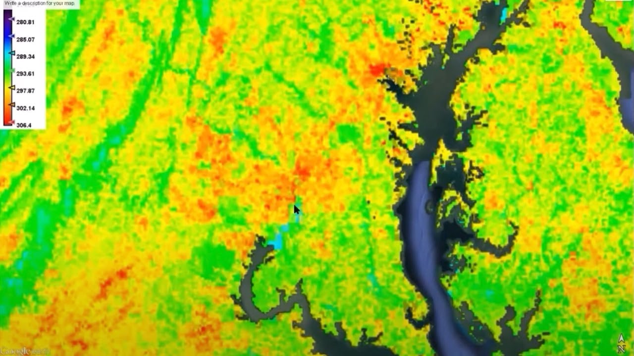
this is the latest collection that we spoke of earlier in the presentation we're going to select the surface temperature band and the quality assessment pixel bound and we're going to filter it and mask it by the function and the variables that we defined above next we're going to filter that collection to any of the landsat scenes that have less than 20 cloud cover and then we're going to print that output to the console window and you'll see that when i run the script when i click run you'll be able to see that next we're going to create a function to apply scaling factors to get the to get the temperature in kelvin and then also to get the temperature in celsius because ultimately what i'm trying to do with this code is if you the temperature land surface temperature in degrees celsius and then again we're going to print that to the console window this is just doing a gut check to know that the code is doing what you want it to do as you're writing it and next thing we're going to do we're going to actually map we're going to define a variable to actually apply those scale factors to that image collection and then this next chunk of code is really calculating the average surface temperature across the landsat collection for those months of july and august so again we're going to create a variable that's going to create the average surface temperature for each pixel across that collection for those two months and then we're going to clip that to the area of interest our study bounds and then we're going to print that and use a print statement so that we can see that the code is working and next thing we're going to do is we're going to select just the surface temperature band and then we're going to define a variable that is going to create a histogram and pass that variable into the histogram so we're only going to display the surface temperature values and we're only going to display those values within the study bounds and this next line of code is actually going to print that histogram so we can see the histogram in the console i like to use histograms because it's a good way of viewing the range of values in this case land surface temperature and it's a good way of just looking at the spread the range of values so you can do statistics and do further analysis or you can also use that for visualization purposes next thing we're going to do is we're going to actually use this map map dot add layer and we're going to add the mapped layer the filtered map layer to the map window and we're going to map we're actually going to display or visualize just the surface temperature using these min and max values and using this palette and we're going to give the map when it appears down here the name surface temperature and we're going to use the display a variable that we defined above saying yes we do want this to display in the map window anytime you run the code this next chunk of code is going to calculate statistics specifically statistics within that average pixel value for july and august for the entire landsat collection with all bad pixels pixels that are cloudy or have cloud shadow all of those have been removed it's the average surface temperature and now what we want to do is we want to take the average temperature just within the urban area and this will help us to be able to derive the urban heat island intensity so this is going to create statistics just for the average within these pixels which is the urban and then the next thing we're going to do is this next line of code is going to take the average for all of the pixels which are in the uh the rural polygons that we created so it's just a way of generating statistics and for both of those we're going to print the results to the console window so we can look at those statistics so when i click run you're going to see that it's going to pan to the to the zoom extent that i defined earlier and it's also going to generate a land surface temperature map of the study area which i delineated the area of interest and it's also showing areas in red which are hot and areas in blue which are are cooler than the the areas in red which are more impervious and built up areas within the map window and it also set the center on the longitude and latitude that we defined and we can see if we zoom into downtown los angeles that we can see that a lot of areas in the downtown area are quite warmer than surrounding areas but we can also see areas like the anacostia river here and the potomac river rock creek park areas of both water and forest greenbelt park here so these natural areas which are more forested or riparian are much cooler than the more built up and especially this downtown area here and in northern virginia here so if i go to the output we can start looking at the histogram here i can actually click on this pop-out and we can do that in a different tab so we can start looking at the spread of values the value on top is actually the degrees in celsius centigrade and we can see the range down below so the range is really from 27 to around 50.
but anyway going back to the code if we drill down a little bit uh deeper we can start looking at the statistics that we output this first one is going to be the min uh mean min and max for the urban area and to drill down to that we're going to click the drop down and we're going to go to features and then zero and then one more time to properties and we can see that we have the surface temperature both the max min and mean i'm interested in the mean because i'm going to use that to derive the surface urban heat island intensity but the other statistics are there as well and again that was for the urban areas in washington which are defined by this polygon here and then next we're going to look at the rural areas and the statistics there which are going to be again if we drill down to features and then zero and then one more time to properties we can see that the we have the main mean and max values for the rural areas that are defined so these are all of the statistics for these four polygons that we defined earlier and again i'm interested in the mean surface temperature which is 30.9 and then to calculate the surface urban heat island intensity what we're going to do is we're going to subtract the the mean surface temperature urban from the mean surface temperature rural and that will give us the surface urban heat island intensity and the intensity of the heat landing is the simplest quantitative indicator of the thermal modification imposed by city upon the geography on which it is situated so this is a really quick way to directly to derive the surface urban heat island intensity for your area of interest now the next code we're going to take a look at is going to look at the landsat time series pixel and we will go to that next the next script we're going to look at will be calculating a time series graph for landsat 8 and 9 at the pixel level the first variable that we see divide is point and that was generated by using the drop a marker which is down here a feature which is down in the map window so we can click on that and we can drop a marker anywhere we want i chose a built-up area in northeast washington dc but you can drop a marker anywhere you want and once we have that we can then define a new variable we're actually going to have to rename that because it'll probably be a generic name like geometry but once we have that we can rename it to point which will be the same nomenclature as we're using in the code here and we'll define a new variable aoi for area of interest and we'll take that point and we're going to buffer that by 30 meters 30 meters is the spatial resolution of a landsat pixel if you were interested in buffering more than 30 meters you could certainly do 60 90 etc it really depends on what level of analysis that you're trying to generate that time series graph of land surface temperature because we're going to be taking the mean of this buffered pixel but again it's really subjective depending on your level of analysis and you can adjust the code you can adjust this parameter to how you want for your own analysis the next chunk of code is to set the base map as the satellite instead of the hybrid or map then we're going to set the map center on a longitude and latitude and use the 12 as the zoom level then we're going to assign a variable for both landsat 9 and landsat 8 bands and we're going to choose the bands for surface temperature and the quality assessment pixel and then we're going to assign new names for those bands that we're going to use later in the script that the variable we're defining is band name and instead of surface temper underscore b10 we'll rename that as just st for surface temperature and we'll keep the qa pixel band name as it is here we will be using the same function the cloud mask function we used in the previous script to remove any cloudy or cloud shadow pixels so we're only going to be doing analysis and time series analysis on cloud free and cloud shadow free pixels then we will create variables l9 and l8 to take the image collection the landsat 9 collection 2 tier 1 level 2 image collection and select just the bands the the land surface temperature and the quality assessment pixel and we're going to filter it by the point the area of interest that point and then also apply that cloud mask and we'll do that for both landsat 9 and landsat 8 collections so that we're working with pixels that actually have values that we're interested in then we're going to create two new variables to pass the filtered collection into and we're only going to collect scenes from that collection that have cloud cover that is less than 20 total in the scene that we're trying to gather if you are in an area say more tropical latitudes that experience more cloud cover you will probably have to change this parameter to something higher than 20 just so you can get scenes that will have pixels of value that you can use so this is very dependent on where your urban area is located so again these are parameters that you will have to change and adjust for your own study area then we're going to use print statements to print the output to the console so that we can do a get check and make sure that our code is actually running the way we want it to next thing we're going to do is concatenate the names of the bands so we want to take the surface temperature underscore with the the name so either l8 or l9 that way when we generate the graph we have a nicely worded graph that has both landsat and landsat 8 and 9 concatenated for just for consistency purposes and next thing we're going to do is merge the collections together so this chunk of code here is taking the filtered landsat 9 and landsat 8 collections based on that one location this is the entire collection so we haven't filtered anything by date these are all the images that are in both collections and they're cloud free and they have good quality pixels and we're going to merge them so instead of having two separate collections we'll just have one collection which we're naming landsat collection landsat coal and that way when we do a time series we just have all of the landsat 9 and 8 together in one collection then we're going to use a create a function same function as we used in the previous code to apply scale factors to generate both both the temperature and kelvin and then also actually just into from kelvin into degrees celsius which is the degree celsius is what i'm most interested in but depending on your analysis you can do either or and then we're going to define a new variable to apply those scale factors to that merged image collection and then again we're going to use a print statement just to make sure that everything is working as i would like it to and lastly we're going to create a new variable time series and in that time series we're going to create a line a line chart and we're going to give that chart a title and give the vertical axis the title and a horizontal axis title and we will be passing in that merged collection of land surface temperature which is buffered to this one point and we're going to print that and when i click run we'll see that all the collections from the print statements are now generated in the console and we also have i can pop this out into a different tab we also have the time series of that merged collection of landsat 8 which is depicted in blue and landsat 9 which are these red dots on the on the right hand side of the graph landsat 8 launched in 2013 so we can start seeing some of the land surface temperature from that buffered pixel and then we can also see because landsat 9 launched in 2021 that's starting in that year we're starting to get some of the land surface temperature from those years as well so this is a really useful way to be able to graph out the land surface temperature for the landsat collection you could take this back further if you wanted to into landsat say landsat 7 landsat 5 and 4. i chose to use landsat 89 because the sensor the thermal infrared sensor is comparable between the two and it's appropriate to use four-level analyses these two sensors together but that is the second script that we're using to show you how to derive a time series for any given location that you're interested in and the last script that i'm going to be walking you through is based on the modis sensor on the aqua satellite and that will be the third script that we'll walk through right now we'll be using the same geometry imports that we used in previous scripts for area of interest rural and urban polygons you can see they've been imported here at the top of the script and then also we have a commented section telling what the script does and then here are the parameters that you'll need to change in the script to adapt this code to your area of interest this first chunk of code is setting the date range by day of year as well as year range as well as defining the study bounds and then also setting defining a variable so anytime we pass this variable into the code below it will appear in the map window we're also centering the map window on the study bounds and then also setting the satellite view as the default base map this next chunk of code is creating a function and we're defining that function by the variable get qc bits and this chunk of code that creates the function is computing the qc bits that we want to extract these qc bits are flag values in each pixel that define pixels that have cloud or cloud shadow or that are flagged for land surface temperature error that we do not want to use later in our analysis so it's going to pull those those qc bits out that we want to extract and this get qc bits we're actually going to be using in this function that we're defining here and this function that we're that we're defining by the name of mask qc this function is going to use the get qcbits function and actually mask out any of the flagged land surface temperature values that have an error or that have cloud or cloud shadow and once we have that function defined we're going to define a variable to get the aqua modis image collection and filter that by the date range the year range and then apply that mask to mask out any of the the flag values for land surface temperature error or by cloud or cloud shadow and then we're going to print the output to the console window next we're going to define a variable for nighttime land surface temperature in celsius and we're going to apply scale factors to derive the pixel in degrees centigrade and we're going to rename the band uh lst night one kilometer to lst night underscore c which stands for land surface temperature at night for celsius and once we have that band renamed and rescaled to degree centigrade we're going to do the same for the land surface temperature in daytime we're going to use this we're going to use this function to create use the scale factors to derive degrees in centigrade and then we're going to rename that band lstd underscore c for land surface temperature in the daytime and in centigrade and then this chunk of code is going to plot a histogram for the number of pixels per location at night that have those land surface temperature values this chunk of code is going to do the same thing it's going to provide account of land surface temperature values per pixel during the daytime and then this chunk of code is going to calculate the average nighttime land surface temperature per pixel across the image collection and then we're going to print that to the console window that way we have land surface temperature the average throughout the entire collection and then we're going to do the same thing for the daytime we're going to take the entire collection from 2010 to 2022 filtered in the months of july and august and we're going to take the average for the land surface temperature across that collection next we're going to print the histogram for those land surface temperature values at night time and we're going to clip it to the study bounds and we're only going to be selecting that the nighttime land surface temperature in centigrade and then we're going to print a histogram so we can view those values in the console window we're also going to do the same thing by plotting histogram values that have been clipped to the study bounds and we're only going to be selecting the land surface temperature in the daytime and centigrade and then we're going to print that histogram again to the console window this next chunk of code is deriving statistics for the mean min and max uh and we're going to be deriving those statistics for the urban area that we delineated that urban polygon so it'll take the mean min and max for that urban core and then we're also going to do the same thing and that's going to be for the mean min and max for the urban area and this is going to be at night time then we're going to derive the statistics for the mean min and max for the rural part of washington dc at night time so that we can derive the surface urban heat island intensity similar to we did in the previous script and we're also going to print both of those outputs to the console window next we're going to do the same thing we're going to be driving statistics for mean min and max except this time it's going to be for the daytime and it's going to be for the auroral areas i'm sorry for the urban and then in this case we're going to be doing the same thing deriving mean min and max for the rural areas in washington dc and then we're also going to print that to the console window so that we can view the statistics and then we're going to add those map layers based on the land surface temperature at night and land surface temperature at daytime and we'll add both of those to the map window so i'll go ahead and click run and we can take a look at the console and you can see that the map window automatically panned to the the area of interest that we defined before and it's also generating see the layers are still generating but we can start looking at some of the results in the console window so we can see that the we have a histogram here of land surface temperature the number of pixels of lamp surface temperature per location at night and we also have a histogram of the number of land surface temperature pixels per location in the daytime and then we also have the output of the the mean of the collection at night time as well as the mean uh across the day and then we also have a histogram of the land surface temperature values at night time so this is the the the range of values at night and then also those range of values of line surface temperature in the daytime again all of these histograms can be popped out into a different tab to be able to view them at a larger scale and then lastly we have statistics this is the the mean min and max of land surface temperature for urban washington dc at night and then the statistics for mean min and max for roar washington dc at night and so if we wanted to calculate the surface urban heat island we would subtract the rural land surface temperature at night time from the daytime and to get those values we can drill down from feature collection to features to zero to properties and then we can see here that the land surface temperature at night for the mean is 21.7 degrees and again this is for the for urban washington dc and then if we want to get the same thing for rural washington dc at night time we can drill down and we can get the mean here that we calculated earlier in the script and this is going to be for again this is for the nighttime rural part of washington dc so we would subtract this value from this value here to get the surface urban heat island intensity at night time and then we also have the statistics here for the mean min and max for urban and rural but this time during the day so this allows us to generate the surface urban heat island for both daytime and nighttime using the aqua modis instrument and then this commented code here at the bottom just explains what i just walked through here in terms of getting those different bands and doing these different equations to have a an intensity of uh surface urban heli island as a quantitative indicator of the thermal modification of a city imposed upon the geography in which it is situated so these are the three scripts to be able to derive time series analysis of land surface temperature as well as to derive surface urban heat island intensity using the aquamodus instrument as well as using the landsat missions as well so now that i've walked through both uh all three of the scripts the we're going to give you some lap time to be able to work with those scripts on your own and we'll be waiting here to answer any questions that you have as you walk through the scripts so again we're giving you roughly 30 minutes to be able to go through those scripts on your own change the parameters for your own area of interest and if you have any questions in the next 30 minutes please do let us know and we'll be here to answer the questions as they come in so we're now giving this time to you to work on calculating your own land surface temperature for your area of interest we will now transition to the question and answer portion of today's webinar we've been getting some terrific questions but if you haven't already please do answer your questions in the q a box we will answer them in the order that they were received we might not get through all of the questions today but we will answer the questions offline and we will post the q a doc to the training website following the conclusion of the webinar below is the contact information for myself as well as my colleague dr amitamekta and we've also provided links to the training webpage and the rset website well we want to thank everybody that's been submitting your questions we've gotten a lot of really great questions and so again we're going to try to get through as many as possible in the next 10 minutes but uh fear not we will answer all of them and we will hope to get this up and posted on the training page within the next couple of days so again if we don't get through all of your questions today don't worry you will be able to find the answer uh sometime later this week so to get into it uh question number one is uh why modis aqua and not also terra and the answer being uh that the modis instrument on the terra satellite only provides land surface temperature estimates during the daytime so if we want to assess urban heat islands uh at night time it's important that we use the aquamodus instrument because it provides products for both daytime and nighttime and that is very useful because a lot of products that you find are especially land surface temperature only provide uh these land surface temperature products during the day and if we want to calculate or assess urban heat island especially during the night time which is very valuable because a lot of times urban heat island effects are more pronounced uh during the night time when the surrounding rural areas cool off uh quite quickly due to the radiative properties of natural vegetation lakes and suburban areas versus the more built up urban area that is very valuable to use the land surface temperature from the modus instrument from the aqua satellite another good reason to use aqua is because the local overpass time for this terra satellite is 10 30 local time whereas with the aqua mission uh the modis instrument on the aqua mission has a local overpass at 1330 and if we're interested in urban heat island effects typically not always but typically land surface temperature will be higher in the afternoon so the aqua mission is better suited for this analysis question number two how did you import landsat to script section so i wasn't exactly sure what this question was asking but if you were trying to access the code we did provide links to you in the chat as well as within the pdf that we're sharing from today's presentation so please try to access the script from there if you're having trouble make sure that you've created a google earth engine account uh using either your gmail or a edu email address and please do refer to the commented sections for each of the areas of the code hopefully they were commented well enough to understand what each section of code is doing but if you are still having problems then do feel free to reach out to me and we can see if we can't troubleshoot uh whatever issue you're having question number three hi all it is fantastic that the code is well commented however is there any documentation for the library that is being used so for all the code that we provided in javascript we use the library functions that come with the google retention api and if excuse me if you're more uh if you want more information on any of the functions that were used you can refer to the documentation which is under the docs tab for each of the different functions that we applied for for each of the three scripts and you can find that yeah the docs tab is on the left hand side of the code editor so hopefully that answered uh the question number three question number four if we change the aoi area of interest by delineating our own rectangle do we have to recalculate the latitude longitude for the uh the function of to set the map center which is map.setcenter and then i suppose otherwise the map display pans to washington dc all the time and that is correct whenever you change the bounding box that rectangle using the draw rectangle tool for your own area of interest then you will need to edit the longitude and latitude degrees and you might have to edit the zoom extent as well depending on how big or small your your urban area of interest is but you will need to change those parameters for the longitude latitude whenever you do change the bounding box that rectangle and rename it to aoi standing for area of interest question number five the script uses the thermal band which is heat reflected what about surface emissivity for landsat does that not contribute to the urban heat on and so one of the surface temperature temperature auxiliary inputs for landsat surface temperature is a global emissivity data set and that data set which is input into the surface temperature algorithm is derived from the advanced spaceborne thermal emission and reflection radiometer it's an aster instrument and that is flown on the terra satellite so surface emissivity does influence urban heat island development it's a measure of surface's ability to shed heat or emit long wave radiation we focused just solely on the land surface temperature alone for deriving surface even urban heat island intensity we did not get into uh any uh uh influences of of emissivity but that's certainly something that that you could look into we were trying to keep it to analysis ready products that you can get uh right in in earth engine and start uh doing analysis and start running applications so that is one of the reasons but but there is an emissivity auxiliary data set that is included in the algorithm to derive the surface temperature question six is there some standard criteria methodology to determine the extension of rural area with respect to the urban area or which is a proportion suggested how do you define the area areas to use as your rural and urban for the calculation of surface urban heat island intensity this is a really great question we got several questions related to this and so hopefully by answering them we will touch upon the questions that were similar that other people would ask but for the for urban areas most people have it's pretty consistent approach to to identifying and delineating urban areas these are pretty much classified as built up planned uh in land cover maps uh as well as uh for urban areas so if you do have access to land cover maps or if you can if you can run an analysis on land surface temperature typically those those higher temperature values that you will find will be especially in in a city will be derived from built up uh impervious surfaces so if you don't have access to a land cover map a uh a a good accurate good excuse a good quality land cover map that is one way to go about delineating urban areas but if you do have access to a land cover map then you can certainly use that to help delineate the those areas google retention does provide global land cover maps some of them at 10 meter spatial resolution those are derived from the sentinel-2 mission from the european space agency so for those that are looking for land cover maps i do suggest looking through the the geospatial data sets through earth engine to to help find those but to get back to the the question though to delineate rural areas in relation to urban areas there are a number of different methodologies uh i would none of them are standardized so i can't speak that anyone is the definitive way some have used different buffering uh methods so once you have that urban core delineated either through your own knowledge of your city or from using land cover maps that you're getting through some other product through other agencies some some methods apply buffer zones from that urban core and that buffer zone can vary and that can vary depending on your area of interest different cities have different suburban sprawl so that will impact how you delineate your rural areas and those buffer zones can range from 1 to 50 kilometers so there is no standard approach in the example provided in the script obviously we delineated rural areas uh based on natural and suburban characteristics that's just for my own knowledge of washington dc which is the city in which i live but for your own area of interest it could be you'll have to place great care in how you select the traits that you want to characterize urban versus rural and we will provide some links to different literature publications that have applied different approaches and we'll certainly give those links before we post this to the the training page so question number seven uh what does the point buffer do does the higher buffer mean a higher analysis area that is correct so anytime you uh buffer the area or increase the uh the spatial scale of that buffer in meters then you are buffering to a larger uh area of analysis so so that is correct so if you if you wanted say a 60 meter buffer or 100 meter buffer or a 120 meter buffer then yeah you would be doing an analysis on that greater area depending on the uh the value of the buffer that you assigned uh question eight is the time of day equal across all images so for all for no i can't say for for nearly all of nasa emissions the local overpass time will be the same so for most sun synchronous orbiting satellites uh and sunseguird as being the aqua satellite the all of the landsat missions are sun synchronous they have the same local overpass time for all the imagery collected for that local for the area of your interest so so the so the time of day will be the same for for for example given in the landsat 8 analysis that we conducted yes it will be as well as for the aquamission there are some nasa missions where the uh the local overpass time will not be the same uh one of those that i'm several i'm thinking of are anything that is might be on the international space station because that does not have a consistent repeat time it has the same orbital swath but the repeat time and the time of day will vary depending on when the imagery is collected i am being mindful the time and i noticed that it is one minute after the the time so we will wrap up here but i will say and i will repeat that for all the questions and we got some wonderful questions that we will be getting to all of them and we will be answering and posting them to the question and answer uh document and we'll post that on the training page hopefully we're shooting for by the end of this week so that it will be ready uh before uh the part three uh which will start next tuesday so again we're having uh you know part two is is going to be in two days so we will post this we will get through all the questions we want to thank everybody for submitting your questions and we also want to thank everybody for joining today uh this is a really important topic uh understanding the urban heat island phenomenon is only going to become more important through climate change and then also being to the ability to be able to characterize and also help mitigate the effects of the urban heat island for those most vulnerable is precisely the topic that we will be covering in part two of this training of this webinar series again part two will be in two days on thursday it will be at the same time we hope that you all join us where we will be able to start learning in part two and then continuing into part three on how you can use different socioeconomic variables to start creating your home your own heat vulnerability indices to help mitigate the effects of what we were characterizing in today's training which is calculating the surface urban heat island intensity so i want to thank the rset team that helped make this possible that's salon hudson odoi jonathan o'brien sarah cutchall and brock blevins as well as my colleague amit demekta so thank you to the rsat team and again i want to thank everybody for joining today and we hope to see you all again on thursday for part two of the webinar series thank you
Up Next
25:42
Urban Heat Islands: Why Cities Are Hotter and How to Cool Them
@pbsterra
415.3K views•2025-06-23

15:54
Life in Biosphere 2: Sustainable Ecosystems & Human Survival
@TED
334.9K views•2009-06-16

93:36
Mapping Urban Heat Islands with Landsat LST in Google Earth Engine
@NASAgovVideo
21.9K views•2020-11-12
10:28
Ice Stupa Artificial Glaciers: Solving Ladakh's Water Crisis
@SonamWangchuk66
3.2M views•2015-05-03
Related Study Plans & Knowledge Roadmaps
Structured learning paths in Environmental Science
environmental-science
Ocean Noise: Cetacean Impacts & Mitigation
01Fundamentals of Underwater Acoustics
02Marine Mammal Bioacoustics
03Anthropogenic Noise: Shipping & Seismic Surveying
+ 2 more learning modules
16h5 modules
Explore Roadmap
environmental-science
Road Ecology: Corridors, Overpasses & Fencing
01Foundations of Habitat Fragmentation and Carnivore Ecology
02The Road Barrier: Ecological Impacts of Transport Infrastructure
03Principles of Ecological Corridors and Connectivity Mapping
+ 3 more learning modules
14h6 modules
Explore Roadmap
environmental-science
Ocean Acidification: Kelp Buffering & Shellfish
01Fundamentals of Ocean Chemistry & pH
02Chemical Pathways of Coastal Acidification
03Bivalve Physiology & Calcification Under Stress
+ 2 more learning modules
18h5 modules
Explore Roadmap
environmental-science
Ice Stupas: Glacial Retreat & Water Security
01Foundations of Glaciology & Mountain Hydrology
02Climate Change and Glacial Retreat Dynamics
03The Science of Ice Stupas & Artificial Glaciers
+ 2 more learning modules
14h5 modules
Explore Roadmap