









![Introduction to Density Functional Theory [Part One] Background](https://i.ytimg.com/vi_webp/Ez_Fm4iTUeo/maxresdefault.webp)







![[APCTP-KIAS School] Prof. Kazuhiro Yabana (Univ of Tsukuba)](https://i.ytimg.com/vi/CYziFOjehms/maxresdefault.jpg)

The Hohenberg-Kohn theorems establish that the ground state electron density uniquely determines the external potential (nuclear positions) and the corresponding wave function, enabling practical density functional theory calculations; the first theorem proves this uniqueness through reductio ad absurdum, while the second theorem shows that the density obeys a variational principle, allowing energy minimization over densities instead of wave functions.
Density Functional Theory: Hohenberg-Kohn Theorems Explained
Added:The many-body Schrödinger equation and the classical wavefunction description of multi-electron systems.
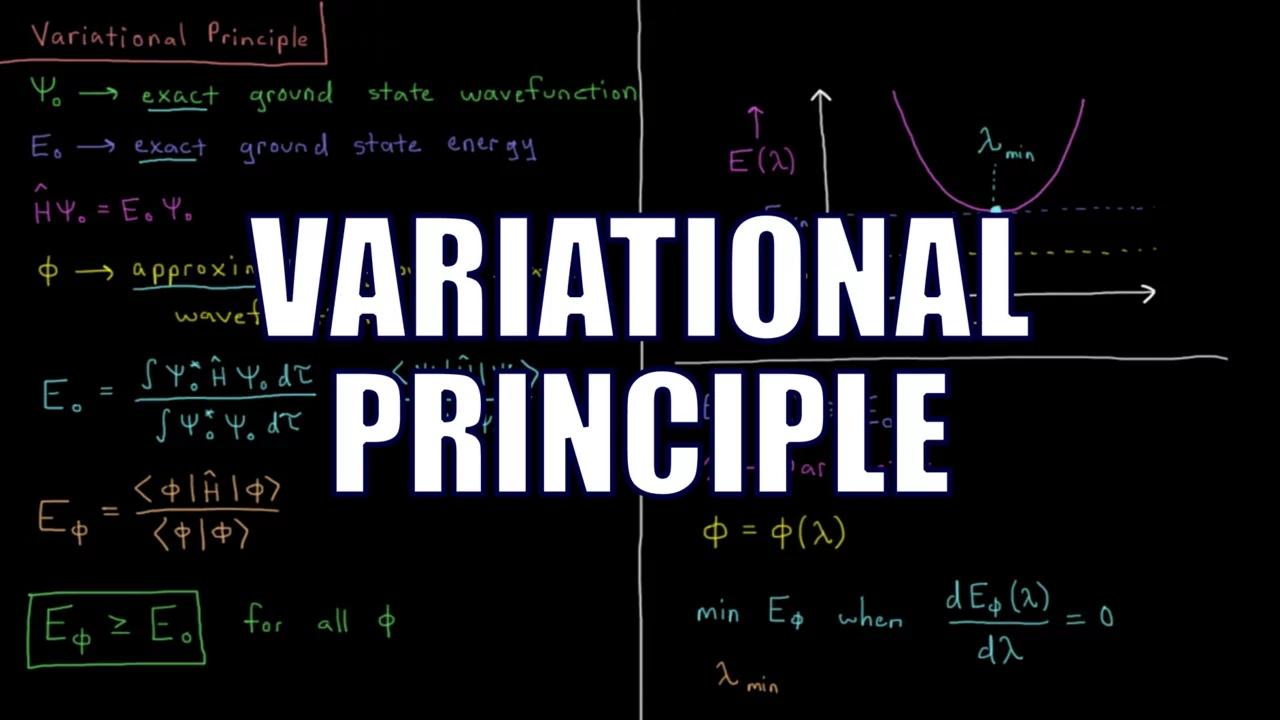
The Variational Principle in quantum mechanics, which establishes how trial wavefunctions relate to ground-state energy.
The mathematical concept of electron density and how it is derived from a many-body wavefunction.
Basic understanding of functional calculus, specifically what a 'functional' (a function of a function) is in a mathematical context.
The Kohn-Sham Equations, which translate the Hohenberg-Kohn theorems into a practical computational scheme using non-interacting reference systems.
Exchange-Correlation functionals and their approximations, such as the Local Density Approximation (LDA) and Generalized Gradient Approximation (GGA).
Practical applications of DFT in computational chemistry and materials science to predict molecular structures, band gaps, and binding energies.
Time-Dependent Density Functional Theory (TD-DFT) for studying excited states and systems interacting with time-dependent fields.
29.5K views347likes12:45Original Release: 2014-06-03
Let's now take a look at the two theorems of Hoenberg and con that led to useful implementations ultimately of density functional theory.
So the rigorous foundation that Hoenberg and Con established in 1964 is based on two theorems. So we'll look at each one, the first one in a bit more detail and just talk about the second one. In any case, recall that density functional theory involves electrons interacting with one another and with an external potential. So that's the language that tends to be used in the physics community. Uh because that potential could be general, but at least in chemistry, external potential effectively only means the potential of the nuclei, the nuclei clamped in their respective positions. So when you hear external potential, you can think of nuclear attraction. Usually the first Hoenberg cone theorem as originally formulated applies to the ground state density of a system and in particular a non- degenerate ground state density. There have been subsequent expansions of the theorem in various directions but we'll just look at that uh initial one. So external potential is the attraction of the nuclei. We get the number of electrons from integrating the density. And what we want to do is show that the ground state density uniquely determines the external potential. All right, that is the ground state density uniquely determines the nuclear positions. And remember that once we know the nuclear positions, there is an exact wave function associated with those nuclei, that number of electrons at those positions. And so if we can prove that a given density uniquely determines an external potential, then we know that there's a mapping relationship between a density and a wave function. So we can map the exact wave function and the exact density. The proof itself actually proceeds via a reductio absorum. And so if you remember how that works in math, you make an assumption. you show that that sum assumption leads to an impossible result and as a result you know that your assumption must have been wrong.
So the hoenber theorem begins then with the following assumption. Assume that there are two different external potentials. So that means two different arrangements of nuclei whether differing in charge or differing in positions or both each consistent with the same non- degenerate ground state density. And so let's uh call those potentials generated by those two different sets of nuclei little va and little vb. And remember that those potentials they determine Hamiltonians H A and HB. So the Hamiltonian would be kinetic energy of electrons, attraction to nuclei uh and repulsion of electrons with one another.
And what would differ of course in A and B would be where the nuclei are for example.
Now for each HA and HB it's an operator.
So each one has a set of igen functions and one of them is the ground state igen function the wave function s0 and it has an igen value e 0 and remember that from the variational theorem we know that if I take the expectation value of h a so that's corresponding to the nuclear positions that give the external potential VA then any wave function I try when I evaluate the energy of that wave function using the Hamiltonian with nuclei at positions A. I will get an energy greater than or equal to in the special case that B were identical to A uh greater than the ground state energy for A.
And so let me just take this inequality and I will specify I'm going to add and subtract HB. So sib the the B I'm actually using here is the ground state energy of the wave function corresponding to nuclear positions at B right and because the external potential uniquely defines the Hamiltonian there is a ground state function for that so in any case that's and that's why I guess I should roll back here one so this is a strictly greater than symbol because I'm not using size 0a a I said that VA and VB are different and as a result the two Hamiltonians are different and they have different uh igen values and igen functions. This is now the ground state function for B evaluated for the Hamiltonian with the nuclei at positions A. So it must be greater than E 0 A because I said my assumption is they're different external potentials.
All right. And uh now I will break up this difference and sum. I'll keep the difference over here. I've just got HB over here.
So the expectation value of the ground state function B for Hamiltonian B is just the ground state value. So I'll just put that igen value in. And then over here I have this term the expectation value of S ground state S for nuclei at positions B of the difference between the two potentials.
Well, this potential the the difference between these two potentials it's it's a one electron operator. Uh and as a result I can write this in a form involving the density. So if I imagine s * s is integrated overall space of density I now have that e the ground state energy of a is less than this difference plus the ground state energy of b. Okay. Okay. Well, this whole thing was just using some arbitrary labels A and B. I could have started back in this last slide labeling this B and this A and this B and this A. Right?
So, I would have gotten the same result that evaluating the other wave function over a given Hamiltonian will give you an energy greater than the ground state for that Hamiltonian.
So, I could just as easily swap all these indices here. So a becomes b, a becomes b, b becomes a and so on. So this also must be true. But if I now subtract n from 10, excuse me, if I add 9 and 10, so I'm going to add this to this, add this to this, add this to this.
So I'll get the sum of the two ground state energies, and then I get this integral plus this integral.
But this is VB minus VA. This is VA minus VB. This is negative this. So this plus negative of this that would all cancel. And I would get that the sum of these two ground state energies is less than the sum of these two ground state energies, but they're the same ground state energies. So that is clearly impossible. You can't have that a plus b is less than a plus b. uh and as a result the assumption must have been incorrect. That is there is not a single density that is associated with both external potentials A and external potentials B. It was that assumption of a single density that allowed us to cancel these two expressions, right?
Because it's the same density appearing in this integral with this difference of potentials. Had we not assumed the same density, everything up till now would have been fine and this would not have canceled. But uh by making that assumption we get this impossible result. And so the first toenber home theorem shows that there is a unique mapping between a given density and its external potential and hence a wave function.
So as long as it's a non- degenerate ground state density and we needed that in order to have that inequality of any expectation value would not be equal to the ground state. uh we determine the external potential, we determine the Hamiltonian, we determine the wave function. And incidentally, remember that the Hamiltonian it doesn't just determine the ground state wave function, it actually determines all the excited state wave functions too, right?
Those are just the other functions of the Hamiltonian.
So that is sort of a a remarkable um uh phenomenon in in some way that the ground state electron density actually determines all the excited states as well. And so you can sort of ask yourself, hm, I wonder what the densities of the excited states might be useful for. And that's still kind of an open question in some areas. But in any case, uh, subsequently the Hoenberg cone theorem has been extended and uh, you can actually show that it applies to the lowest energy non- degenerate state within each irreducible representation of the molecular point group. So that's a little bit of a group theory thing and it extends it from just uh the ground state to other uh states as well that that may u may be of interest in certain systems but we won't explore that too much further.
Now the second Hoenberg cone theorem follows from the first. The first is an ex an existence theorem. Basically, it says or maybe I shouldn't even call it an existence theorem. Rather, it is a proof of the relationship between the density and the wave function that there's a 1:1 mapping. What it doesn't tell you is how to get the density that uh is exact for a system. So, how do we go about that? Well, the second Hoenber cone theorem shows that the density obeys a variational principle. And just as with MO theory, we're always trying to optimize the energy to drive it down lower. And so Hoenber and Con said that given a well-behaved density that integrates to the proper number of electrons, we know that theorem one says that density determines a candidate wave function. Right? There is a unique mapping of a density to a wave function.
We can evaluate the energy of that candidate wave function over the Hamiltonian corresponding to the density and we will get some value for the energy that is and we know that it must be greater than or equal to the exact value because the exact value only comes from the exact density which determines the exact Hamiltonian and the exact wave function. So that is a an almost trivial proof in some sense that there is a variational principle and it also offers you an operational approach to identifying this best density that is in principle choose different densities that satisfy an external potential. And so remember the external potential that's the nuclear positions. So we need a density that has the right sort of cusp behavior and the right uh uh uh gradient spherically averaged gradient of the density at the nuclear positions. But of course there's a lot of freedom in the other positions not not those exactly at the nuclei. So we could just keep varying our density a bit subject to those constraints and as we drive energy down and down by constantly checking uh by taking each of those densities and coming up with a corresponding wave function and Hamiltonian uh you would get closer and closer to correct. But how do you choose these improved densities? That's you know the first question. It's a little sounds like it would be sort of a pain to just be randomly varying the density at all positions in space. Moreover, part of the goal is not to have to solve a shreddinger equation. That sounds quite unpleasant. As a matter of fact, we've we've shown that there is a mapping, but we haven't exactly said how to accomplish that mapping. And in indeed, you might imagine it would be a bit tricky. Well, in in particular, figuring out the kinetic energy seems like it might be a bit tricky. So how can the density be used in a variational equation to determine the energy without recourse to the wave function? That is really what chemistry is waiting for in order for the big breakthrough of DFT starting to be employed by your average everyday theoretician in his or her laboratories with his or her micro computer. So in the next uh lecture we will take a look at the first practical applications.
Up Next
59:12
Kohn-Sham Equations Explained | DFT Theory Tutorial
@teachingthetheoryindensity7936
9.7K views•2017-06-12

83:56
Biocatalysis and Catalysis in Islatravir Synthesis | Merck Webinar
@SCIwheresciencemeetsbusiness
675 views•2020-10-08

20:08
Potential Energy Surfaces Explained | Computational Chemistry Lecture
@ChemProfCramer
82.3K views•2014-06-03

17:31
Edible Water Bottles: A DIY Guide to Sodium Alginate Spherification
@ryan
10.5M views•2019-06-21
Related Study Plans & Knowledge Roadmaps
Structured learning paths in Chemistry
chemistry
Nuclear Chemistry: Decay, Meds & Fuel Cycle
01Introduction to Nuclear Structure and Radioactivity
02Decay Dynamics and Kinetics
03Radiation Interaction and Detection
+ 2 more learning modules
24h5 modules
Explore Roadmap
chemistry
Supramolecular Chemistry: Forces & Machines
01Foundations of Chemical Bonding and Intermolecular Forces
02Introduction to Host-Guest Chemistry
03Thermodynamics and Dynamics of Self-Assembly
+ 2 more learning modules
16h5 modules
Explore Roadmap
chemistry
Photochemistry: Excited States & Reactions
01Foundations of Light-Matter Interactions
02Molecular Orbitals and Electronic States
03Photophysical Processes and Jablonski Diagrams
+ 2 more learning modules
18h5 modules
Explore Roadmap
chemistry
Coordination Chemistry: Bonding & Properties
01Introduction to Transition Metals and Ligands
02Crystal Field Theory (CFT) and Geometry
03Magnetic Behavior and Spin States
+ 2 more learning modules
14h5 modules
Explore Roadmap