This video demonstrates how to implement a PID (Proportional-Integral-Derivative) controller using Arduino for a BAR 30 pressure sensor, providing a technical solution for controlling pressure systems with precise feedback mechanisms.
Arduino PID Controller for BAR30 Pressure Sensor Guide
Added:Deep Dive
Basic Arduino programming and hardware interfacing, including using external libraries and uploading code via the IDE.
Arduinoya Giriş-Sıfırdan Arduino Öğreniyorum#1
51.4K
This section teaches Arduino IDE navigation and fundamental programming concepts. The IDE includes File menu for project management, Library Manager for adding external libraries, Tools menu for board and port selection, and Serial Monitor for debugging. Arduino programs use two main functions: void setup() for one-time initialization and void loop() for continuous execution. Pin configuration requires pinMode() to set pins as INPUT or OUTPUT. Digital output control uses digitalWrite() with HIGH (5V) or LOW (0V) states. The delay() function creates time delays in milliseconds (1000ms = 1 second). LEDs require current-limiting resistors to protect them from excessive current and extend operational lifespan.
Click to watch →
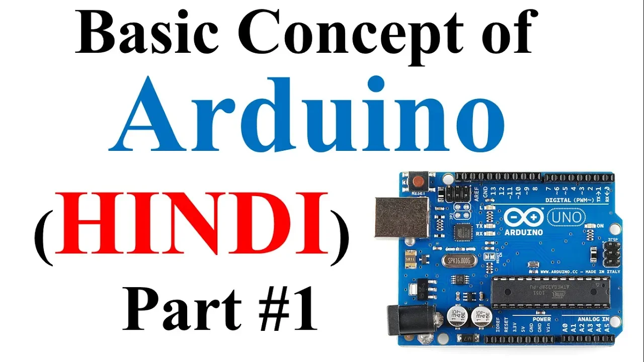
Basic concept of Arduino in Hindi | Arduino tutorials for beginners part #1
1.4M
Arduino IDE is free software available for all operating systems (Windows, Mac, Linux). Download from Arduino website by searching 'Arduino IDE' and clicking the first official option. After installation, the desktop icon launches the IDE containing: File menu (New, Open, Save), Examples menu with pre-written code templates (LED blinking, LCD interfacing, sensors), Sketch menu with Include Library for sensor commands, and Tools menu for board and port selection. For successful programming, select the correct board (Uno, Mega, Nano, Mini) and the connected serial port (e.g., COM3). The Upload button transfers programs to Arduino, enabling control of connected components like the built-in LED on pin 13.
Click to watch →

Introduction to Arduino IDE
525
Arduino IDE is an open-source Integrated Development Environment for programming Arduino microcontrollers, compatible with Windows, Linux, Mac, and Android (via Arduino Droid). The interface includes File menu with Sketchbook (stores user programs) and Examples (provides pre-written code samples). Libraries are imported using #include <library_name.h> syntax. Before uploading, users must select the correct board type (Uno, Nano, Mega) and USB port. The IDE provides Verify and Upload buttons for code management. Arduino programs consist of void setup() (executes once) and void loop() (executes repeatedly). Digital pins range from 0 to 13. Variables are declared using 'int variable = pin_number;' syntax. pinMode(pin, mode) configures pins as INPUT or OUTPUT. digitalWrite(pin, state) sets pins to HIGH (on) or LOW (off). delay(milliseconds) pauses execution, where 1000 milliseconds equals 1 second.
Click to watch →

الدرس -2- برنامج Arduino + برمجة اول مشروع
22.2K
The Arduino IDE consists of four main sections: Menu bar, Toolbar, Code editor, and Console. Key functions include: File operations (New, Open, Save, Print), Code editing (Cut, Copy, Paste, Find, Go to Line), Code verification (Check for errors), and Code upload (Ctrl+U). The IDE supports both Arabic and English languages. Libraries extend functionality for specific hardware or protocols, available through the Library Manager. External libraries can be downloaded from the internet and added via Sketch > Include Library > Add .ZIP Library.
Click to watch →
كيف تدخل عالم برمجة الأردوينو في ١٠ دقائق | Arduino Coding in 10 Minutes
5.8K
Arduino components share common pin configurations: positive (VCC), ground (GND), and signal (SIG) pins. Signal pins function as INPUT for sensors or OUTPUT for devices. Arduino has 14 digital pins and 6 analog pins. Jumper wires (M-F, M-M, F-F) enable connections. Breadboards facilitate prototyping with internal metal conductors. Circuit diagrams show logical connections; implement on breadboard by connecting components in sequence. Replace battery with Arduino: connect GND to circuit negative, digital output pin to circuit positive. Arduino programs have three sections: Setup (initialization, runs once), Loop (main logic, runs continuously), and Variables. Key functions: pinMode() configures pins, digitalWrite() sets HIGH/LOW states, delay() pauses execution. Code executes sequentially; use variables for pin numbers to avoid repeated code. Upload code via USB after selecting board and port.
Click to watch →
Deep Dive
Fundamental concepts of closed-loop feedback control systems, specifically the theoretical roles of Proportional, Integral, and Derivative (PID) controllers.

Understanding PID Controllers: Proportional-Integral-Derivative Explained
232.6K
This section establishes the theoretical foundation of control systems and introduces proportional control. A PID controller, developed by Nicholas Minorsky in 1922, is a control structure used in closed-loop systems that compares input and output to generate control signals. Control theory deals with dynamic systems, and the 'plant' refers to the system being controlled (originating from Industrial Revolution terminology). Open-loop systems lack feedback and cannot compensate for disturbances, while closed-loop systems measure output and provide feedback. The proportional controller multiplies error by a constant (KP) to produce output, but this creates steady-state error where the system never exactly reaches the set point because zero error produces zero output. The integral controller addresses this by accumulating total error over time, mathematically corresponding to finding the area under the error curve.
Click to watch →
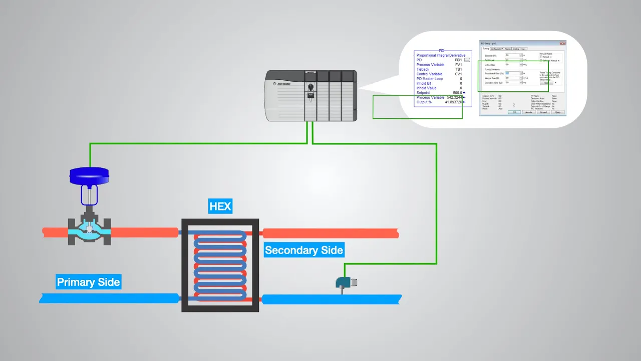
PID Controller-Introduction with Details and Comparison with P, PI & PID #bms
15.2K
The PID controller is the most widely used closed-loop control system, combining Proportional (P), Integral (I), and Derivative (D) components. P generates output proportional to current error, I sums error over time to eliminate steady-state error, and D predicts future error based on rate of change. These three components work together to provide stable control with zero steady-state error, fast response, and no oscillations. The mathematical expression includes gains Kp, Ki, and Kd for each component respectively.
Click to watch →
TIA PORTAL TP35: Régulateur PID pour SIMATIC S7-1200/1500 ( PID Compact )
28.4K
This section covers the foundational concepts of closed-loop control systems and PID (Proportional-Integral-Derivative) regulation. A closed-loop system consists of four key components: setpoint (desired value), comparator (error calculation), regulator (control logic), and actuator (executive element). The PID controller combines three distinct actions: proportional action provides immediate correction proportional to current error, integral action eliminates steady-state error through time accumulation, and derivative action anticipates future errors by responding to rate-of-change, thereby improving system stability. These principles form the theoretical basis for industrial automation and process control applications.
Click to watch →

Intro To Controls
276
The closed loop transfer function is T(s) = G(s) / (1 + G(s)H(s)), where the denominator is the characteristic equation. Poles determine stability: left half-plane poles indicate stable systems. PID controllers (Proportional, Integral, Derivative) are widely used because they are simple, robust, and effective. The proportional term responds to error magnitude, the integral term eliminates steady state error, and the derivative term anticipates future errors. Proportional controllers decrease rise time but cause steady state error and amplify noise. Integral controllers eliminate steady state error but can cause actuator windup. Derivative controllers reduce overshoot but amplify high frequency noise. Root locus plots show how poles move as gain varies.
Click to watch →

Source Code, Fraud Algorithms, and Injecting Votes: Dr. Daugherity - "Let My People Go" Interview
1.4K
A PID controller is a closed-loop feedback system consisting of three components: Proportional (P) responds immediately to current error, Integral (I) accumulates past errors to ensure complete correction, and Derivative (D) predicts future errors based on current rate of change. Using cruise control as an example: P applies immediate gas adjustment when speed drops, I remembers any remaining deficit to apply gradual correction, and D anticipates hills or declines to prevent overshooting. The combination creates stable, responsive control without excessive oscillation.
Click to watch →
Deep Dive
Understanding of the I2C communication protocol, which is the physical and logical interface used by the BAR30 pressure sensor.

Arduino Boost Gauge, 2025 edition
44.8K
Connect I²C pressure sensor to Arduino: SCL to pin A5, SDA to pin A4, VDD to 5V, GND to ground. Two pins are NC (not connected). The sensor measures pressure from -100 to +300 kPa (approximately -1 to +3 bar). Use Wire library for I²C communication instead of bit-banging.
Click to watch →
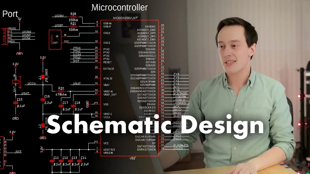
Schematic Design - Landing Model Rockets Ep. 4
176.9K
I²C (Inter-Integrated Circuit) is a serial communication protocol using two lines: SDA (Serial Data) and SCL (Serial Clock). Multiple devices can share the same bus by using unique addresses. The processor communicates with sensors like the IMU and barometer over this bus, allowing multiple sensors to be connected with minimal wiring.
Click to watch →
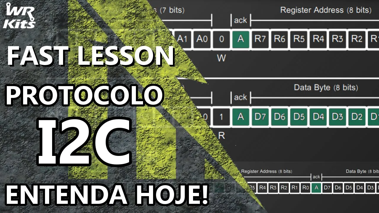
ENTENDA O PROTOCOLO I2C EM POUCOS MINUTOS!
24.7K
The I2C (Inter-Integrated Circuit) protocol, developed by Philips in the 1980s, is a synchronous two-wire communication interface (SCL for clock, SDA for data) that enables a single master device to communicate with multiple slave devices within an electronic system. The protocol operates at frequencies typically between 100 kHz and 400 kHz, with some devices supporting up to 5 MHz. Communication begins with a Start condition (SCL high, SDA falling edge) and ends with a Stop condition (SCL high, SDA rising edge). Data transfer involves sending a 7-bit slave address followed by a read/write bit, with slaves responding via acknowledgment (ACK) or non-acknowledgment (NACK) signals. For writing, the master sends 8-bit data to a specific register; for reading, the master initiates a Restart condition, sends the same address with a read bit, and the slave transmits 8-bit data back. External pull-up resistors are required due to the open-drain configuration of the bus lines.
Click to watch →

I2C Protocol Explained: A Technical Overview of Serial Communication
227.5K
I2C (Inter-Integrated Circuit) is a widely-used synchronous serial communication protocol developed by Philips in 1982 that enables short-distance data transfer between devices using only two wires: Serial Data (SDA) and Serial Clock (SCL). The protocol operates in a master-slave architecture where the master initiates communication by sending a start condition, followed by the 7-bit slave address and a read/write bit, then exchanging data bytes with individual acknowledgments from the receiver, and terminating with a stop condition. Key technical aspects include the open-drain configuration with pull-up resistors (typically 1-10kΩ) that determine bus speed, and support for multiple operating modes ranging from Standard Mode (100 kbps) to Ultra-Fast Mode (5 Mbps).
Click to watch →
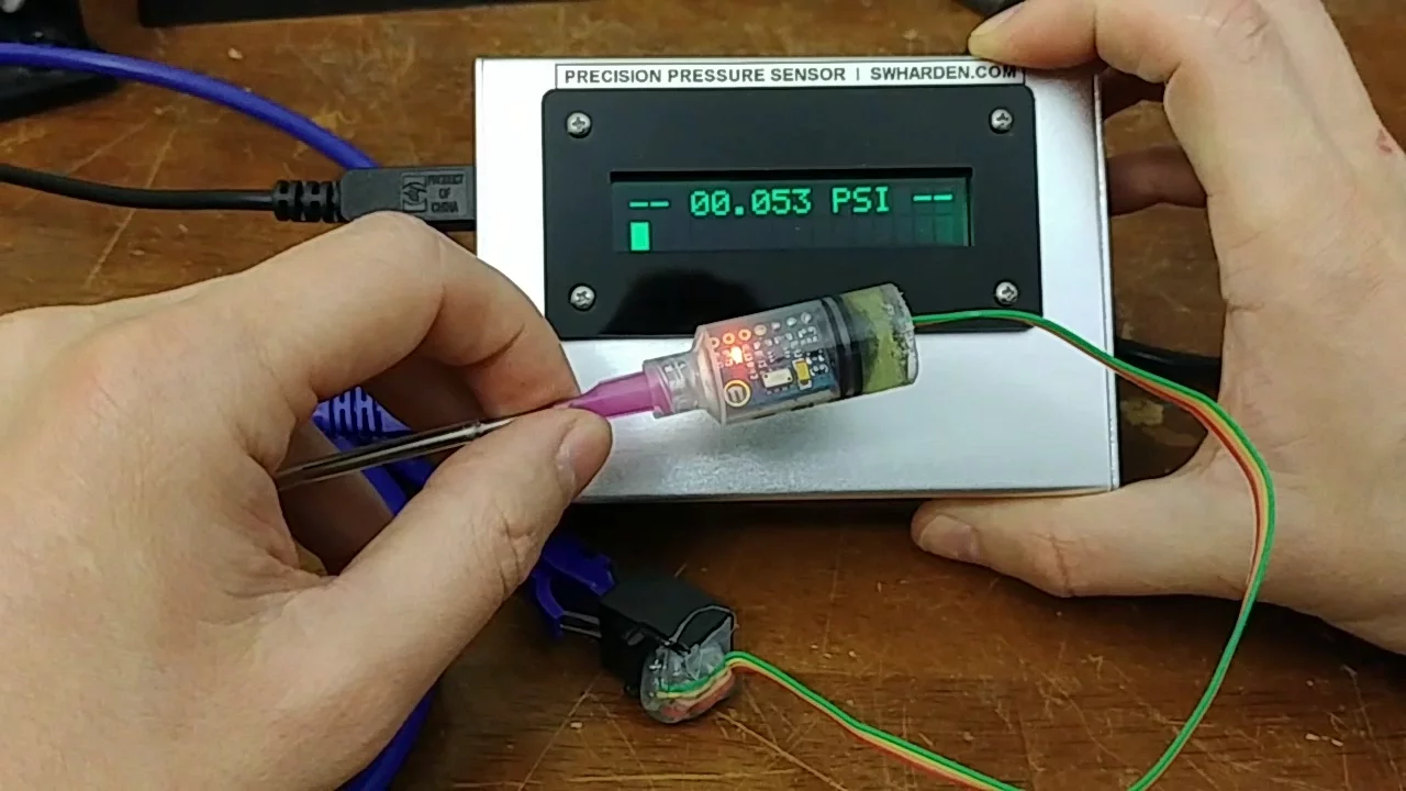
Precision Pressure Meter Project
23.3K
This comprehensive section covers I²C communication principles and device interaction. Topics include: (1) the two-wire I²C protocol using clock (SCL) and data (SDA) lines; (2) device addressing with the MS5611 found at address 0xEE; (3) understanding the five basic commands: reset, program memory read, D1 conversion (temperature), D2 conversion (pressure), and ADC read; (4) scanning I²C buses to identify connected devices; (5) configuring the Bus Pirate for I²C mode at appropriate speeds; (6) enabling power and pull-up resistors for reliable communication; and (7) establishing a foundation for manual sensor interrogation.
Click to watch →
Deep Dive
The physical relationship between hydrostatic pressure and depth in fluid mechanics to interpret BAR30 sensor readings correctly.
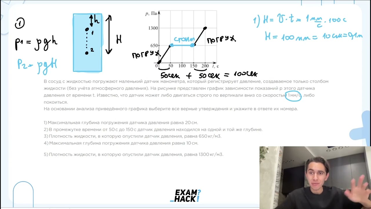
В сосуд с жидкостью погружают маленький датчик манометра, который регистрирует давление - №23167
438
Hydrostatic pressure increases linearly with depth according to the formula P = ρgh, where ρ is fluid density, g is gravitational acceleration, and h is depth; by analyzing pressure-time graphs and knowing the sensor's velocity, one can determine the depth profile and calculate fluid density from pressure readings at specific depths.
Click to watch →
Como funciona uma sonda de nível hidrostática? | VIVER DE PLC
5.7K
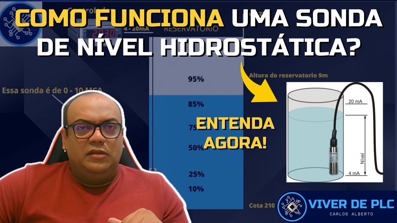
There is a direct relationship between water column height and pressure: every 10 meters of water column produces approximately 1 bar of pressure. This relationship allows conversion between pressure measurements and liquid level. The bar is a common unit for measuring pressure, though other units like PSI or kg/cm² are also used. Understanding this relationship is fundamental for interpreting hydrostatic sensor readings.
Click to watch →

حل النماذج الاستراشاديه -حل نماذج الوزاره -فيزياء تانيه ثانوي ٢٠٢٦ |متبقاش جهاز
200.8K
This segment covers pressure-depth relationships (P = P₀ + ρgh), barometer readings and atmospheric pressure, and hydraulic press force calculations. The instructor demonstrates how to calculate pressure at different depths in fluids, how to interpret barometer readings to determine atmospheric pressure, and how to calculate forces in hydraulic systems using the area ratio principle (F₁/A₁ = F₂/A₂).
Click to watch →

حل النماذج الاسترشادية في الفيزياء | الصف الثاني الثانوي 2026
1.2K
Pressure in a fluid increases with depth according to P = P₀ + ρgh, where P₀ is surface pressure, ρ is fluid density, g is gravitational acceleration, and h is depth. The slope of a pressure-depth graph equals ρg. To convert between units, divide Pascals by 10⁵ to get bars. The intercept on the pressure axis represents the surface pressure.
Click to watch →

La fórmula de la presión hidrostática PASO A PASO.
284
The hydrostatic pressure formula P = ρgh calculates the pressure exerted by a fluid at a given depth, where ρ is fluid density, g is gravitational acceleration, and h is depth; this explains why pressure increases with depth and is independent of container shape or volume, allowing calculation of maximum depth for waterproof devices like watches rated at 10 BAR (1000 kPa) which can withstand approximately 102 meters of water depth.
Click to watch →
Prerequisite Knowledge
- Concept 01Basic Arduino programming and hardware interfacing, including using external libraries and uploading code via the IDE.
- Concept 02Fundamental concepts of closed-loop feedback control systems, specifically the theoretical roles of Proportional, Integral, and Derivative (PID) controllers.
- Concept 03Understanding of the I2C communication protocol, which is the physical and logical interface used by the BAR30 pressure sensor.
- Concept 04The physical relationship between hydrostatic pressure and depth in fluid mechanics to interpret BAR30 sensor readings correctly.
Subsequent Learning
- Step 01Advanced PID tuning methodologies, such as the Ziegler-Nichols method or software-assisted autotuning, to optimize controller response.
- Step 02Implementation of signal filtering techniques (e.g., Kalman filters or low-pass filters) to mitigate sensor noise and prevent derivative kick in the PID loop.
- Step 03Integrating the pressure-based PID controller into multi-thruster autonomous underwater vehicle (AUV) firmware for stable depth-hold capabilities.
- Step 04Exploring cascade control system architectures where the depth PID loop provides a setpoint for a velocity or thruster control loop.
Facing Problem
Video Purpose
Core Solution
Key Techniques
Further Guidance
Final Advice
Facing Problem
0:08Playing Section
- 1
Starts addressing viewers facing a difficult situation.
- 2
Sets context of needing a solution quickly.
Limitations of Linear PID and the Need for Robust Control with Sensor Fusion
While a standard PID controller on a basic Arduino is an accessible starting point for BAR30 pressure sensor integration, it has significant limitations in real-world underwater applications. Linear PID controllers struggle with the highly non-linear dynamics of underwater environments, such as thruster deadbands, tether drag, and changing currents, often leading to instability or sluggishness. Furthermore, raw pressure readings from the BAR30 are highly susceptible to noise from thruster wash and wave action. Relying solely on basic Arduino hardware restricts the implementation of advanced noise-filtering and estimation algorithms, such as Kalman Filters. Control system experts argue that robust control strategies—like Sliding Mode Control (SMC) or Model Predictive Control (MPC)—combined with multi-sensor fusion (integrating IMU and pressure data) on 32-bit microcontrollers are necessary to achieve stable and precise depth control in practical underwater vehicles.
Deep Dive
Advanced PID tuning methodologies, such as the Ziegler-Nichols method or software-assisted autotuning, to optimize controller response.

PID Tuning with the Ziegler-Nichols Method: A Tutorial
377.6K
The Ziegler-Nichols method provides two empirical approaches for determining PID controller gains: the first method uses the step response curve's inflection point to calculate L (distance from origin to tangent) and T (vertical distance), then applies formulas (KP=0.9T/L, KI=1.2T/L, KD=0.075L); the second method involves increasing proportional gain until the system exhibits sustained oscillations at critical gain Kcrit and period Pcrit, then using formulas (KP=0.5Kcrit, KI=1/(1.2Pcrit), KD=0.125Pcrit) to determine controller parameters. Both methods are simple to implement but have limitations and work best for certain transfer functions.
Click to watch →
Understanding PID Controllers: Proportional-Integral-Derivative Explained
232.6K
Manual PID tuning involves: setting Ki and Kd to zero, increasing Kp until oscillation occurs, then increasing Ki to correct steady-state offset, and finally adjusting Kd to eliminate oscillations. Alternative methods like Ziegler-Nichols reduce trial-and-error requirements. Modern PID controllers use code on microcontrollers rather than discrete components. Key applications include automotive cruise control (originally researched for ship steering), manufacturing equipment, and reflow ovens for precise temperature control during soldering processes.
Click to watch →
![ZIEGLER NICHOLS ✅ SEGUNDO Método [Control PID] Parte 2](https://i.ytimg.com/vi_webp/AAaWNNuqpuY/maxresdefault.webp)
ZIEGLER NICHOLS ✅ SEGUNDO Método [Control PID] Parte 2
109.1K
The Ziegler-Nichols Method 2 is an experimental technique for tuning PID controllers by first determining the ultimate gain (Ku) and ultimate period (Pu) through proportional-only control until sustained oscillations occur, then applying empirical formulas to calculate the proportional, integral, and derivative gains; this method requires the closed-loop system to have third-order dynamics or contain time delay to achieve oscillatory behavior, and while it provides a starting point for controller parameters, fine-tuning is typically necessary for optimal performance.
Click to watch →
Designing a PID Controller Using the Ziegler-Nichols Method
187.3K
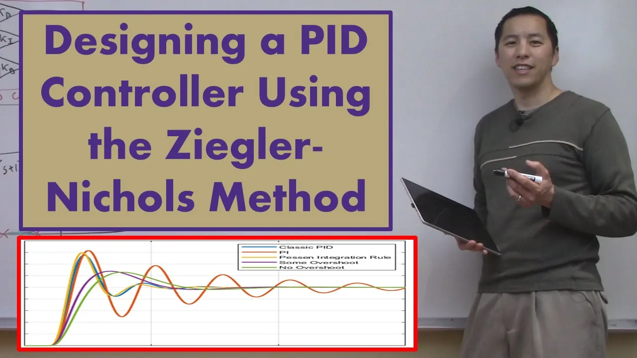
The Ziegler-Nichols method is an iterative online technique for tuning PID controllers that requires no mathematical model of the plant; the procedure involves starting with proportional-only control, gradually increasing the proportional gain until the system reaches neutral stability (oscillations at constant amplitude), recording the ultimate gain (Ku) and ultimate period (Tu) of oscillation, and then using empirical formulas to calculate the PID gains: KP = 0.6Ku, TI = Tu/2, and TD = Tu/8 for classic PID control. This method provides a practical starting point for controller design but has limitations including lack of mathematical rigor, requirement for initial system stability, and potential cost/danger when applied to expensive hardware.
Click to watch →

Comment déterminer les paramètres d’un correcteur PID : la première méthode de ZIEGLER NICHOLS
36.8K
The Ziegler-Nichols first method is an empirical technique for determining PID controller parameters by analyzing the step response of a first-order system: after identifying the inflection point and drawing a tangent line, the time delay (L) and settling time (T) are measured, then the controller gains are calculated using specific formulas (Kp = 0.9×T/L for P, Kp = 1.2×T/L and Ti = L/0.6 for PI, and Kp = 1.2×T/L, Ti = L/0.6, Td = 0.5×L for PID), which can be implemented and validated through MATLAB simulation.
Click to watch →
Deep Dive
Implementation of signal filtering techniques (e.g., Kalman filters or low-pass filters) to mitigate sensor noise and prevent derivative kick in the PID loop.
Evitando Ruídos no PID (na prática)
614
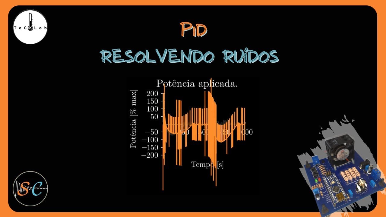
In PID controllers, the derivative term amplifies high-frequency sensor noise because its gain increases with frequency; to make the derivative causal and implementable, a low-pass filter (P/(s+P)) is added, and the filter parameter P should be chosen using the rule P = N/TD where N is between 8-20 and TD is the system time delay, to balance noise filtering with maintaining desired closed-loop dynamics.
Click to watch →
Noise Filtering in PID Control | Understanding PID Control, Part 3
398.5K
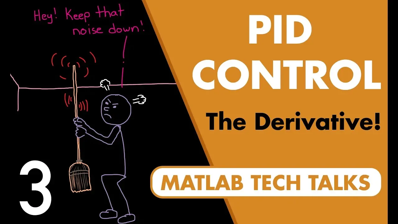
In PID control systems, the derivative term amplifies high-frequency noise from sensors, which can destabilize the controller even when the noise amplitude is low; to mitigate this, a low-pass filter is applied to the derivative path, blocking high-frequency noise while allowing the lower-frequency control signal to pass through, with the filter's cutoff frequency determining the balance between noise rejection and signal fidelity.
Click to watch →

Control Theory Seminar - Part 3
20K
Derivative kick occurs when applying a step input to a PID controller, causing an impulse (infinite spike) in the derivative term because the derivative of a step is an impulse. This causes undesirable spikes in the control effort. To eliminate derivative kick, commercial PID controllers apply the derivative action to the plant output rather than the error signal. Additionally, filters are typically placed on the derivative path to limit high-frequency gain (since differentiators have infinite gain at infinite frequency).
Click to watch →
Controladores PID avanzados
259
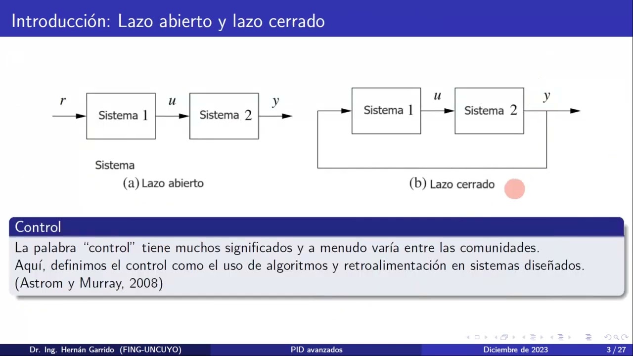
The derivative term amplifies measurement noise because high-frequency noise has large derivatives. To prevent this, the derivative is implemented as a filtered derivative: Kd*s/(τs + 1), where τ is a filter time constant. This filter attenuates high-frequency noise while preserving derivative action at lower frequencies. The cutoff frequency ωf = 1/τ should be higher than system dynamics frequencies but lower than noise frequencies. At frequencies much lower than ωf, the filter has minimal effect (gain ≈ 1); at higher frequencies, it strongly attenuates the signal. Second-order filters provide steeper attenuation for very noisy systems.
Click to watch →

Meetup 9 Aspectos generales del PID y sus aplicaciones en microcontroladores
307
Derivative action has two critical limitations: noise amplification and derivative kick. Noise amplification occurs because real signals contain noise, and the derivative of noisy signals produces large values that can destabilize the system. Derivative kick occurs when reference changes suddenly, causing infinite derivative values and large control spikes. Solutions include adding first-order low-pass filters to the derivative term and calculating derivative from output rather than error. These practical considerations are essential for robust PID implementation in real-world systems where noise and reference changes are inevitable.
Click to watch →
Deep Dive
Integrating the pressure-based PID controller into multi-thruster autonomous underwater vehicle (AUV) firmware for stable depth-hold capabilities.

Design of Depth Keeping AUV
283
This video presents a senior capstone project where Cory Nalis designed and built a depth-keeping Autonomous Underwater Vehicle (AUV) from scratch, learning skills in electrical design, system integration, software development, and project management; the AUV uses an ESP32 microcontroller with a custom PID controller to maintain depth within ±5cm accuracy using a B2 pressure sensor and BNO055 IMU, featuring four brushless thrusters arranged for simplified kinematics and a streamlined acrylic housing with 3D-printed components.
Click to watch →

So baust du dein erstes U-Boot in Stormworks
358
The depth hold system automatically maintains a set depth using a PID controller. The presenter creates a microcontroller with inputs for activation, target depth, and current depth. A memory register stores the target depth value. The presenter demonstrates using an advanced PID controller with proportional gain (P), integral gain (I), and derivative gain (D) values. Starting with P=1 and I=0, D=0 provides basic operation. The presenter adds a small offset to allow manual override when needed—pressing W or S temporarily pauses the depth hold system. A clamp limits minimum depth to zero, preventing the system from trying to maintain negative depths. The depth hold system works effectively, maintaining the submarine at the target depth despite wave action.
Click to watch →

From The Depths | Submarine Tutorial! | All the basics!
47.7K
Submarines can be built using two main depth control systems: air pumps that fill sections with air to control buoyancy (simple but unreliable as breaches flood the section), and PID (Proportional-Integral-Derivative) controllers that automatically adjust thrusters to maintain a set depth; for stability, propellers should be matched to the center of mass, and redundant control systems are recommended for reliability, with propulsion typically consisting of forward-facing thrusters for movement and side-mounted thrusters for turning.
Click to watch →
From the Depths: Stream 1b
117
PID (Proportional-Integral-Derivative) control systems can replace multiple separate ACB components in vehicle design, creating unified control systems for pitch, altitude, and roll. This integration improves stability and reduces the need for expensive thrusters. Each axis can have different modifiers based on position within the craft. The system demonstrates how PID controllers can make previously unstable vehicles perform reliably, with the ability to handle aggressive maneuvers like full-power pitching while maintaining stability.
Click to watch →

Sonar Guided Torpedo Tutorial - Step by Step Guide - Stormworks
46.1K
Implementing autonomous movement requires integrating propulsion with control logic. Basic forward motion uses constant number blocks connected to motor outputs, with Ctrl key enabling multi-selection for efficient wiring. Depth hold implementation employs PID controllers comparing altitude sensor readings against setpoints. Key parameters include proportional gain for immediate response, integral gain for error correction, and derivative gain for damping oscillations. Standard starting values (P=0.2, I=0.001, D=5) require tuning based on vehicle weight and fin configuration. This demonstrates how feedback control systems enable stable autonomous operation in dynamic environments.
Click to watch →
Deep Dive
Exploring cascade control system architectures where the depth PID loop provides a setpoint for a velocity or thruster control loop.

This is what a Master's degree in Robotics Engineering Looks like
38.2K
Cascade control uses nested PID controllers where an inner controller regulates one variable and an outer controller regulates another. For the robot, the inner PID (running at 100 Hz) regulates the roll angle, while the outer PID (running at 10 Hz) regulates the robot's velocity. The outer PID takes the target velocity from the joystick and outputs the target angle for the inner PID, which then outputs the final wheel velocity.
Click to watch →

My Engineering Thesis is Imploding
10K
Motor controllers use cascade PID structure: current loop (innermost), velocity loop (middle), and position loop (outermost). Position commands translate to velocity, then current, processed by Field Oriented Control (FOC) for efficient torque generation. Each controller has P, I, D parameters requiring tuning. Velocity tuning: increase gain until motor turns poorly, then reduce by 50%. Position tuning: find critical oscillation point and slightly reduce gain. Velocity integrator gain is typically 10× velocity gain. The most common technique is systematic guess and check.
Click to watch →

Rebuilding a Balancing Robot with Position and Velocity Control
171.9K
This section covers advanced control techniques beyond basic balancing. Position hold allows the robot to maintain a specific location by averaging encoder readings from both wheels to determine actual position, then using a PID controller to modify the balance setpoint toward the target. A cascaded control architecture with two PID loops eliminates oscillations seen in single-loop implementations. When encoder readback introduces latency, velocity hold becomes preferable by monitoring the PID controller's own output instead of reading back encoder values. This approach achieves similar results to position hold without communication delays. Both strategies demonstrate how control system architecture significantly impacts robot performance and responsiveness.
Click to watch →

Emerson DeltaV | PID Cascade Control P53 | LAB Test Procedure
1K
Cascade control involves two interconnected PID controllers where the output of the master controller serves as the setpoint for the slave controller. In this lab demonstration, PID1 operates as the master controller in manual mode while PID2 functions as the slave controller in cascade mode. When PID1's output is manually adjusted (e.g., to 60%), PID2's setpoint immediately updates to match. When both controllers operate in their respective cascade modes (PID1 in auto, PID2 in cascade), the system can respond to setpoint changes from the master controller. The flow loop (slave loop) responds quickly to follow the setpoint, while the master loop (temperature loop) reaches steady state more slowly, demonstrating how cascade control enables rapid response to disturbances in fast loops while maintaining stability in slower master loops.
Click to watch →
Điều khiển truyền động điện - Chương 2 phần 6 MS Teams online
2K
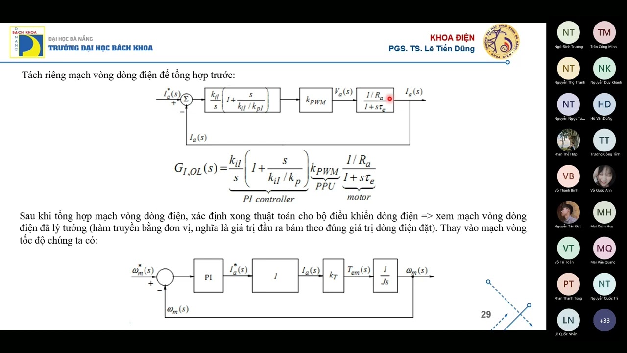
Cascade control systems with position, speed, and torque loops require hierarchical synthesis from innermost to outermost loops. The innermost loop (torque/current) has the fastest processing speed, while the outermost loop (position) has the slowest. Electric drive systems require mathematical models separated into electrical and mechanical parts: electrical part takes voltage input and produces current/torque output, while mechanical part takes torque input and produces speed output. The position loop is obtained by integrating speed over time. Controllers use PI structures based on error feedback, with the innermost loop suitable for optimal control modules. The correct synthesis order is from inside out, as designing outer loops first leads to incorrect system behavior.
Click to watch →
Facing Problem
Video Purpose
Core Solution
Key Techniques
Further Guidance
Final Advice
Facing Problem
0:08- 1
Starts addressing viewers facing a difficult situation.
- 2
Sets context of needing a solution quickly.
Limitations of Linear PID and the Need for Robust Control with Sensor Fusion
While a standard PID controller on a basic Arduino is an accessible starting point for BAR30 pressure sensor integration, it has significant limitations in real-world underwater applications. Linear PID controllers struggle with the highly non-linear dynamics of underwater environments, such as thruster deadbands, tether drag, and changing currents, often leading to instability or sluggishness. Furthermore, raw pressure readings from the BAR30 are highly susceptible to noise from thruster wash and wave action. Relying solely on basic Arduino hardware restricts the implementation of advanced noise-filtering and estimation algorithms, such as Kalman Filters. Control system experts argue that robust control strategies—like Sliding Mode Control (SMC) or Model Predictive Control (MPC)—combined with multi-sensor fusion (integrating IMU and pressure data) on 32-bit microcontrollers are necessary to achieve stable and precise depth control in practical underwater vehicles.
Basic Arduino programming and hardware interfacing, including using external libraries and uploading code via the IDE.
Fundamental concepts of closed-loop feedback control systems, specifically the theoretical roles of Proportional, Integral, and Derivative (PID) controllers.
Understanding of the I2C communication protocol, which is the physical and logical interface used by the BAR30 pressure sensor.
The physical relationship between hydrostatic pressure and depth in fluid mechanics to interpret BAR30 sensor readings correctly.
Advanced PID tuning methodologies, such as the Ziegler-Nichols method or software-assisted autotuning, to optimize controller response.
Implementation of signal filtering techniques (e.g., Kalman filters or low-pass filters) to mitigate sensor noise and prevent derivative kick in the PID loop.
Integrating the pressure-based PID controller into multi-thruster autonomous underwater vehicle (AUV) firmware for stable depth-hold capabilities.
Exploring cascade control system architectures where the depth PID loop provides a setpoint for a velocity or thruster control loop.
126 views1likes3:05@RoelVandePaarOriginal Release: 2021-10-28
[Music] morning youtubers so here it's about 8 a.m at your place it might be like 2 am and you're facing this difficult issue and you just want to get out of the office what are you doing in the office at 2am anyway um this video will try and help you out technically i hope you subscribe to my channel and that you like the video that will really help me and my family out god bless [Music] so [Music] do [Music] do [Music] so [Music] [Music] do [Music] please click subscribe and like thank you thank you for watching and may god bless you always
Up Next

19:09
Why 'Yes' Means 'No' in East Asian Communication
@aini_
354.1K views•2024-08-16

12:54
Triumph of Orthodoxy Icon: Byzantine Art & History Explained
@BenCallan
2.1K views•2024-08-06

9:49
FastAPI vs Flask vs Django: Choosing the Right Python Web Framework
@TechWithTim
302.5K views•2024-05-26

1:42
Game of Thrones Opening Credits: A Cinematic Analysis
@gameofthrones
46.3M views•2011-04-18
Related Study Plans & Knowledge Roadmaps
Structured learning paths in General & Interdisciplinary Studies
general-studies
Elevator Engineering: History, Physics & Cities
01From Hoists to Safety Brakes: The Dawn of Vertical Lift
02Hydraulic vs. Traction: The Engineering Physics of Elevators
03Modern Speed, Safety, and Algorithms
+ 2 more learning modules
12h5 modules
Explore Roadmap
general-studies
Rubber: Material Science, History & Geopolitics
01Origins of Natural Rubber & Mesoamerican History
02The Chemistry of Natural Rubber & Vulcanization
03The Geopolitics of the Rubber Boom & Colonization
+ 2 more learning modules
12h5 modules
Explore Roadmap
general-studies
Containerization: Evolution, Logistics & Trade
01Ancient Trade & Bulk Cargo: Amphorae to Barrels
02The Industrial Revolution & Cardboard Packaging
03The Containerization Revolution: Malcom McLean
+ 2 more learning modules
12h5 modules
Explore Roadmap
general-studies
Textile Tech: Evolution, Labor & Global Impact
01Pre-Industrial Textiles: Handloom & Cottage Industry
02Mechanization: The Spinning Jenny to the Power Loom
03The Factory System & Global Labor Transformation
+ 2 more learning modules
10h5 modules
Explore Roadmap