






![[Hindi] Python Matplotlib Tutorial - Python Data Science and Big Data Tutorials](https://i.ytimg.com/vi_webp/VFsRLjSc8GA/maxresdefault.webp)





![Guide to Kerbal Space Program...for Complete Beginners! - Part 8 [Maneuver Planning to Minmus]](https://i.ytimg.com/vi_webp/CnkrUU8zTPw/maxresdefault.webp)











The gravitational sphere of influence (SOI) of a planetary body is defined as the region where the gravitational acceleration from that body dominates over the gravitational acceleration from the central star (like the Sun), and it is calculated by setting the ratio of perturbing acceleration from the central body to the central body's own acceleration equal to the ratio of perturbing acceleration from the perturbing body to the perturbing body's own acceleration; this concept is essential for switching between different gravitational reference frames during spacecraft trajectory propagation, such as transitioning from heliocentric to planetocentric modeling when a spacecraft approaches a planet like Jupiter.
Gravitational Sphere of Influence | Orbital Mechanics with Python
Added:Newtonian Mechanics and the Law of Universal Gravitation, including gravitational acceleration and force equations.
The classical Two-Body Problem and Kepler's Laws of Planetary Motion to understand standard orbital trajectories.
Basic Python programming, specifically familiarity with numerical libraries like NumPy and plotting tools like Matplotlib.
Elementary vector mathematics and coordinate systems used to define positions and velocities in 2D/3D space.
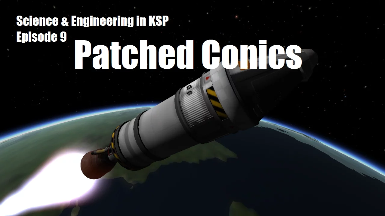
The Patched Conic Approximation method for calculating interplanetary trajectories by joining multiple two-body orbits.
The physics of Gravity Assists (slingshot maneuvers) to understand how spacecraft exchange momentum with planets.
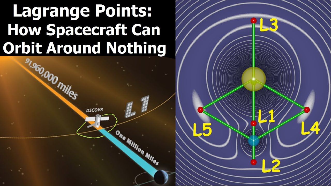
The Three-Body Problem and N-Body simulations, exploring chaotic systems and Lagrangian points where SOI simplifications break down.
Spacecraft Trajectory Optimization techniques, such as designing transfer orbits (e.g., Hohmann, bi-elliptic) using advanced Python packages like poliastro or Astropy.
3.6K views90likes9:39Original Release: 2021-05-02
the gravitational sphere of influence of a planetary body can be used for approximating when one body's gravity like the earth or jupiter dominates over the body that it itself is orbiting which is the sun and note that this isn't an exact value and there are multiple accepted definitions of this value like the planetary sphere of influence and the hill sphere and this can be used to switch the center of propagation when getting close to planetary bodies like when a spacecraft is approaching jupiter when it gets close enough you want to switch the propagation from being modeled as a heliocentric elliptical orbit to a jupiter hyperbolic orbit and it can also be used to switch from modeling a planetary system as a berry center like the jupiter berry center or as modeling each body separately like modeling jupiter separate from its moons like callisto europa and io and this video will be using the voyager 2 flyby of jupiter which is seen on the left here as an example to illustrate how the gravitational sphere of influence is defined there's a 40 second video in the series and this one will be going over the n-body perturbations the ratio of the m-body perturbation to central body gravity which is how the sphere of influence is defined and we'll be using the voyager 2 flyby of jupiter as an example to visualize all of these equations and if you haven't seen already on this channel i have the space engineering podcast and videos in spanish and if you stick around to the end of the video here i'll show how i plugged this equation here into python in order to show how to define the sphere of influence of a body here we'll do a quick overview of the end body perturbation but if you'd like a more detailed analysis going into the geometry of the end body perturbation i'll have a link in the description to a video i made a while back on it so in the two body problem of orbital mechanics we model one larger body to be the center of the gravitational force that a smaller body is influenced by in this case the larger body would be the sun and the voyager true spacecraft in the smaller body who is orbiting the sun the two body problem gives us an equation of the acceleration of the small body due to the large body's gravitational pull which is a function of the mass of the large body and the vector pointing from the large body to the small body we can then model the gravitational force of other bodies as a perturbing force onto the spacecraft which in this case would be jupiter as a perturbing body so here we are using the voyager 2 spacecraft doing a flyby of jupiter and we have two different scenarios on the first one on the left we are modeling the sun to be the central body and jupiter is a perturbing body in this case we have some acceleration due to the sun as a central body and some perturbation from the gravity of jupiter and in the case on the right we model jupiter as a central body and then the perturbation is coming from the sun's gravity we can then define these ratios of how large the perturbing acceleration is from each body as compared to the central body acceleration and the sphere of influence of a body jupiter in this case is defined where these two separate ratios are set equal to each other so when we model the sun as a central body the ratio of jupiter's gravitational perturbation to the sun's gravitational acceleration is equal to when we model jupiter as a central body the ratio of the sun's gravitational perturbation to jupiter's central body acceleration and this is where the sphere of influence comes from at the position of the spacecraft when these two ratios are equal to each other now going back to the equations defining the accelerations of the central body and the perturbing body we have these two equations where the acceleration due to the larger body is newton's universal law of gravitation and then the perturbing body acceleration is a modified version of that equation so we have here that these equations are a function of the vector pointing from the sun to the spacecraft and also the vector pointing from the sun to jupiter and then the vector pointing from the spacecraft to jupiter we can then use those equations and expand out this ratio equation to have the full form equation of how we're going to be able to calculate the gravitational sphere of influence here are the results of plugging in voyager 2's jupiter flyby trajectory to that ratio equation so on the right we see the 3d trajectory of the flyby with the cyan part represents when voyager 2 is outside of jupiter's sphere of influence then the purple part is when voyager 2 is inside jupiter's sphere of influence and for the plots on the left the red ratio jupiter is the ratio equation when jupiter is modeled as a central body and the yellow ratio sun is when the sun is modeled at the central body so we can see as voyager 2 is coming in the point where the two ratios are equal which is the green dot here is when voyager 2 is coming into the sphere of influence here and then exiting on the point of the right here which corresponds to that point here and then the reason why this ratio sun has this massive large spike right in the middle is because the perturbation acceleration due to jupiter's gravity as seen in this equation here is over a thousand times more massive than the acceleration due to the sun since voyager 2 is so much closer to jupiter at that time and jupiter is a very massive body so here is the python script that i use in order to create that ratio plot so we have the typical imports numpy spicy pie matplotlib planetary data i just need to get in order to get the mu values of the sun and jupiter so we start out by furnishing the necessary spice kernels which the solar system kernel just has a leaf seconds kernel and then d432s.bsp in order to get the decisions of jupiter over time and then jpl has published the voyager 2 and voyager 1 bsp kernel so i'll have link in description where you can find that to find an initial date of 1979 may 1 turn that into ephemeris time and then propagate for some amount of time create an array of ephemeris times and then some empty arrays and the important part here is that for each ephemeris time so for each time step we want the sun to spacecraft vector the jupiter to spacecraft vector and then the sun to jupiter vector and we have here that the spice id of voyager 2 is negative 32 in this bsp kernel we have whatever premise time it is the j2000 frame and then 10 is the spice id for the sun and then 5 is the spice id for the jupiter berry center in this case we get the sun mag which is just the magnitude of the acceleration of the sun when it is modeled as a central body which is just the simple equation same thing jupiter the magnitude of jupiter's acceleration when it is modeled as a central body and then we have the magnitude of the sun when it is modeled as a perturbation same thing jupiter when it's modeled as a perturbation and then plug in all those values into the arrays do a little bit of math here find the arguments so that where the minimum between them is the smallest which is when they are equal and then print out a bunch of stuff and then doing the plot is actually pretty straightforward just typical matplotlib stuff here uh nothing too fancy but basically the math here is this important part just getting all the vectors using spice.spk geo and make sure you load the necessary spice kernels and then it's pretty much the same thing for doing the 3d plots this is no longer to do because i finished it so yeah same thing with the 3d plots in this case you want to import the spacecraft i did animate orbits but you don't have to do that obviously orbit calculations spice tools basically it's all the same thing just define some initial time some final time create an array of those ephemeris times calculate all the ephemeris for voyager 2 with respect to the jupiter berry center create a norm of all the r's spear of influence all that good stuff and then just pass it into the plot orbits function and then plot states function i was using it one time but i didn't actually end up eating it but the important part is the plot orbits here which i have the plot orbits function in the astro dynamics with python repository so you can go ahead and use that i haven't implemented the sphere of influence which i guess i can just show right now if we go to python tools plotting tools and then so plot euler's plot quads omegas this is for the spacecraft attitude control stuff we get to plot orbits uh we have central body sphere of influence if we want to use it the color the alpha and then to plug it in we have right here so if this argument is not none so this is this is going to be a number so what is a central body sphere of influence like a value of kilometers and then plotting that as a wireframe because i made a post a while back uh comparing if i want to do like a like um a sphere or a wireframe and you all voted that you preferred the wireframe so i just implemented the wireframe like that it's actually pretty straightforward not too difficult to plug in but yeah let me know if you want me to put this in the github repository just plug in this part right here so be sure to hit like and subscribe to help me out with youtube algorithm and to keep up to date with all the new videos on this channel and let me know in the comments if you have any questions about this video if anything was unclear and i'll be going over the hill sphere influence in another video so the next video is going to be sphere of influence propagation stop conditions where you can plug in to the spacecraft class when to check if you've exited a sphere of influence of the central body or if you've entered the sphere of influence of another body and that's going to be very useful when i then go into the next video getting to patch conics and how to do patch conics types of propagation so again let me know any questions or comments that you have and thank you for watching
Up Next

5:09
Gravity Assist Speed Calculation: Physics Explained
@Ingenium_dr
621 views•2025-06-09

12:53
21cm Hyperfine Transition in Neutral Hydrogen: Radio Astronomy Basics
@AaronRobertParsons
12.4K views•2011-10-13

10:10
Hohmann Transfer Calculations: Earth to Mars and Venus | Orbital Mechanics with Python
@alfonsogonzalez-astrodynam2207
11.1K views•2020-11-16

27:14
Entropy and the Second Law of Thermodynamics Explained
@veritasium
27.5M views•2023-07-01
Related Study Plans & Knowledge Roadmaps
Structured learning paths in Physics
physics
Nuclear Physics (Decay, Fission & Reactors)
01Atomic Structure and the Binding Force
02Radioactive Decay and Half-Life
03Nuclear Fission Mechanics and Chain Reactions
+ 2 more learning modules
12h5 modules
Explore Roadmap
physics
Soft Matter (Polymers, Colloids & Rheology)
01Foundations of Soft Matter & Thermal Forces
02Polymer Physics and Macromolecules
03Colloids, Surfactants, and Self-Assembly
+ 2 more learning modules
38h5 modules
Explore Roadmap
physics
Analytical Mechanics: Lagrangian & Hamiltonian
01Mathematical Foundations: Calculus of Variations
02From Newtonian Mechanics to Constraint Dynamics
03The Principle of Least Action & Lagrangian Mechanics
+ 3 more learning modules
28h6 modules
Explore Roadmap
physics
General Relativity (Spacetime & Cosmology)
01Foundations of Relativity: Special Relativity
02The Geometry of Spacetime: Equivalence Principle & Curvature
03Einstein's Field Equations: The Mathematics of Gravity
+ 2 more learning modules
55h5 modules
Explore Roadmap