










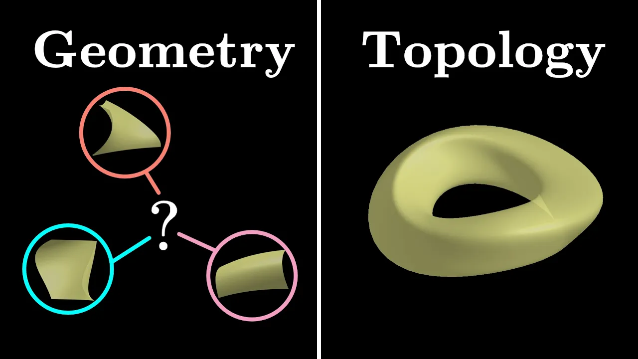




The second fundamental form is a symmetric bilinear form on the tangent plane of a surface, defined as II(v, w) = -v · dn(w), where dn is the differential of the Gauss map (shape operator). This form encodes how the surface bends in space and has eigenvalues called principal curvatures (κ₁, κ₂) whose product gives Gaussian curvature (K = κ₁κ₂) and average gives mean curvature (H = (κ₁+κ₂)/2). Gaussian curvature distinguishes surface types: positive K indicates elliptic (bowl-shaped) surfaces, negative K indicates hyperbolic (saddle-shaped) surfaces, and zero K indicates parabolic (cylindrical) surfaces. Mean curvature measures how the surface interacts with its normal vector.
Shape Analysis Lecture 6: Surface Curvature Fundamentals
Added:Multivariable Calculus: Proficiency with surface parametrization, tangent planes, and computing surface normal vectors.
Linear Algebra: A strong understanding of eigenvalues, eigenvectors, and symmetric bilinear forms, which are crucial for analyzing the shape operator.
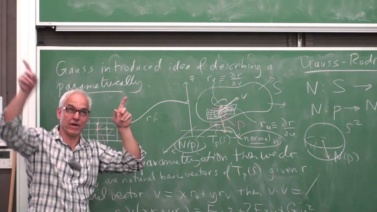
First Fundamental Form: Familiarity with the metric tensor, arc length, and how distances and angles are measured on a parameterized surface.
Differential Geometry of Curves: An understanding of curvature, torsion, and the Frenet-Serret frame for one-dimensional space curves.
Theorema Egregium: Exploring Gauss's landmark theorem which proves that Gaussian curvature is an intrinsic property of a surface.
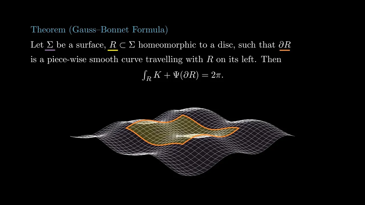
The Gauss-Bonnet Theorem: Understanding the profound connection between a surface's local geometry (curvature) and its global topology (Euler characteristic).
Minimal Surfaces: Studying surfaces with zero mean curvature, including physical applications like soap films and mathematical modeling.
Discrete Differential Geometry and Computer Graphics: Applying these curvature concepts to discrete triangle meshes for 3D shape segmentation, processing, and rendering.
8.6K views189likes1:11:15Original Release: 2021-04-15
hello everybody and welcome to our next lecture of 6838 today we're going to embark upon a series of two two and a half lectures that cover one of the most classic topics in both theoretical and applied differential geometry like if you take a totally theoretical differential geometry undergraduate course uh over in the math department you'd spend a lot of time on this topic and in the applied world we'll spend a lot of time on it too because it's just that important and that topic is computing the curvature of surfaces so essentially our goal for these lectures is going to be to quantify how a service deviates from flatness so remember that a surface is a locally two-dimensional object but essentially our last lectures that were just defining surfaces really were mostly topological in nature we're just defining what it means to be a surface now in today's lecture now that we know what it means to be a surface we want to know how to distinguish one surface from another and we're going to start by doing that with the most classical approach which is by computing curvature curvature is exactly what it sounds like it's a measure of bendiness and we'll see that there are two really important notions of curvature on a two-dimensional surface embedded in 3d those are gaussian curvature and mean curvature and these two curvatures sort of quantify all the different ways that a two-dimensional surface can bend through three-dimensional space unsurprisingly both of those curvatures are going to equal zero when the surface is flat because flat things don't have curvature so there are all kinds of high-level questions that we can answer when we go about trying to compute curvature so for instance we're going to be able to use our curvature measures to distinguish at different points on a surface by the way this can change from place to place between bowl-shaped surfaces like the top uh parabolic surfaces like the middle and hyperbolic surfaces like the bottom as we see on the slide here we're going to see that those three classes are easily distinguished by a particular measure of curvature called gaussian curvature on the other hand we can also see kind of how the surface interacts with this normal vector like does it bend toward or away from the normal vectors like the first two images that we see on the top here and we're going to see that that is largely quantified by a second notion of curvature called mean curvature and this question of how to distinguish different types of surfaces shows up all over the place when we start analyzing geometry so for instance a sort of related question we could ask is how does a surface interact with space so here i show you a piece of origami i would say a pretty boring piece of origami where it's essentially just a flat sheet that i've creased a few times and then bent into space now the key word here and one that we often use informally but rarely do we think about it formally in mathematical terms is bent we bent the flat surface to achieve the surface on the right now in our course when i say band what i'm going to mean is that i deformed that flat surface without changing its distance structure so in particular let's say that i'm an ant crawling along that sheet of paper and so when the paper is bent you know if the ant crawls along and it just moves along the bend the ant cannot distinguish between the left and the right cases so in other words if all the ant knows how to do is to compute distances along the surface these two surfaces are identical now obviously the way i've rendered it here these are not identical surfaces right one of them is completely flat and one of them is bent over and so essentially ants can't distinguish bending of surfaces they can only distinguish stretching and so what we're going to see is that one of our notions of curvature is largely designed to detect this style of deformation which kind of really has to do with the interaction between the surface and the space around it and then another one where like maybe i just stretch out my surface like a piece of rubber is going to be associated to a different notion of curvature so in fact this sort of theme of like does the surrounding space matter one that we originally raised in our very first lecture in 6838 is going to keep coming back over and over and over again in particular what we're going to show is that the surrounding space really doesn't matter for one notion of curvature called gaussian curvature but it does for mean curvature we're going to see that in a variety of different ways in both the discrete and the smooth cases and of course we're going to talk about many practical applications my favorite one that i saw on the internet is that once you understand surface curvature you can optimize the way that you eat a piece of pizza according to science uh apparently we've all been doing it wrong so i'll uh refer you guys to this article here for additional detail on this groundbreaking application of surface curvature now the first thing we have to do is think about what our approach should be how should we go about quantifying the bendiness and the stretching of surfaces that are sitting in 3d and one way to do it that i think is kind of a reasonable approach given what we've done so far is to go back to the case of curves so recall that we've already talked about curvature and a different notion of bending is called torsion when we discuss the differential geometry of smooth curves remember that the curvature of a curve kind of is like the steering wheel direction of a car as it drives along the curve in a plane then the torsion is kind of how the curve lifts out of a plane and we spent quite a bit of time very carefully defining these two notions so what we're going to do in today's lecture is basically to leverage what we already constructed for curves and lift it to the surface case so the way that we're going to do that intuitively is actually pretty straightforward we're going to think about drawing curves with the restriction that the curves only can live along the surface they can't you know they're like paths of a car driving along some bendy landscape and essentially what we're going to see is that the curvature vector of that path that path which is restricted to move along the surface has certain structure that we can use to describe the surface itself rather than the path and in fact that's actually pretty intuitive so for instance let's say that i'm driving a car along a bumpy piece of terrain right so as i drive my car it goes up and down and up and down notice that if i were a passenger in the car and i closed my eyes i could sense the fact that my car is moving along the terrain right there's acceleration which is essentially due to the fact that the ground underneath the car is changing and that has to do with the ground it actually doesn't have to do with my car right there's no way to drive along a curved landscape and not feel some force which is due to just keeping you on the ground and so essentially what we're going to see is that that force is roughly the curvature of the surface in a given prescribed direction and so we're going to formalize all these notions of course but really that's all that's going on again that if i can drive a car with constant speed along a surface then i can sense the curvature of that surface which is pretty cool okay so we'll first recall a few notions from the last few lectures just to make sure that we all are on the same page then we're going to dive right into some computations definitions and a bunch of stuff in between so let's get started so of course the main thing that we're going to make use of today is the unit normal to a surface now recall that only orientable surfaces have unit normal fields globally but even non-orientable surfaces have unit normal fields at least locally so we can always do this in some small patch on a surface although computing one global field of normals may be impossible so today we're going to think of the normal as little n which is a function from the surface m into the unit sphere right and the reason i say it's from the surface into the unit sphere is that of course normals are unit length vectors okay so essentially we've got this notation that we separate set up in our previous lecture right a normal is going to be little n we're going to use t sub p to denote the tangent space at a particular point p and m is going to stand for manifold but today we're in the two dimensional domain so m is always going to be a two dimensional manifold or surface moreover we're not going to worry about manifolds with boundary for now in fact defining curvature on a boundary is a little bit of a tricky matter and you have to decide whether it's important for a particular application or not so this is a pretty typical thing to omit so if you'll recall when we talked about the analysis of plane curves we defined a particular object called the gauss map which mapped every point on a plane curve to its normal vector in this case on the circle which is s1 now we're going to lift the gauss map to a surface sitting in 3d which now is going to map to the unit sphere which is notated s2 and then finally as a last little bit of review here recall that we essentially define curvature in terms of this object we called the frenet frame which is essentially measuring how the tangent normal and binormal vectors of a curve change in response to the curve uh deviating from flatness so what we're going to do is leverage some of the measurements here to define curvature for a surface sitting in 3d now if any of these terms is a little unfamiliar or still uncomfortable that's okay we're going to try and recall them as we go through today's lecture and the great thing about having video lectures is of course that you can go back and watch it again and make sure that you have the right intuition okay so let's get started so as i've already mentioned the basic object that we're going to work with today is an object called the gauss map gauss by the way his name shows up all over the place there's a gauss map there's gaussian curvature he's a big guy when it comes to differential geometry so the gauss map of an oriented surface is a map from the surface into the unit sphere which is just giving the unit normal to every point on that oriented surface notice that an oriented surface i guess has kind of two choices of gauss map whether the normal points outside or inside we're just going to assume that somebody has has oriented the surface meaning they have chosen a normal direction n and you know the convention is usually that n is pointing outward assuming that your surface is closed and has an inside so we're going to need one additional notion which we've already introduced in past lectures and that's the differential of a map in fact we've defined it a few different ways because we first talked about the differential of a scalar function and then we lifted it to a differential of a more general map between spaces so just as a tiny review remember that if phi is a map from m into n here both m and n can be sub manifolds then we can define the differential d phi at a point p as follows where essentially what we're going to do is take any curve gamma whose tangent is a given vector uh at that point p and we're going to say that essentially d phi in the gamma prime direction is nothing more than the rate of change of phi as gamma walks through the curve so again if you're uh unfamiliar with this definition i know that essentially i'm skipping over it a little bit in the most general case i refer to the course notes or to some of the previous lectures to get an intuition for what this d object is doing but d here really just stands for derivative this is just a glorified way to multiply by the jacobian matrix of a uh map so the first thing that we're going to do uh is actually compute the differential of this map from the surface into the unit sphere notice the unit sphere is actually a manifold right you know the unisphere is just a ball and so it makes perfect sense to compute dn at a point p and this object has a name this is called the shape operator okay so we're going to draw a little bit of a schematic and then we're going to prove a nice little lemma which is going to be convenient for the remainder of today's lecture so let's hide our slide in the corner here and get started with a little bit of a computation so first let me draw a bit of a picture just to recall uh what's going on we're going to see a lot of tour i in today's lecture because honestly that is the only oriented surface without a boundary that your instructor knows how to draw okay so let's uh let's go ahead and do that so here is a taurus you make it a double taurus by putting two of these things there and remember that again the normal map we're going to use little n by the way i'm going to use big n and big t for like the normals and tangents of curves i'm going to use little n and maybe little t for normals and tangents and surfaces we'll see that big n and little n are going to be different it's pretty rare that the tangents are different that's that's okay so anyway uh right so our gauss map goes from our surface into the unit sphere which is notated s2 by the way this is a piece of notation that always trips people up if you have the unit sphere in 3d right so this is sitting in r3 then it's notated s2 by the way i guess these axes should be right at the center of the sphere but whatever uh and essentially the reason for that is that it is a two-dimensional surface right it's intrinsically 2d even if it's sitting in 3d right so in general you have like s n minus 1 sits in rn right so this is like r 3 here and remember that essentially all n does is maps every point to its normal okay so now the question is what is this object dn so what does it mean to differentiate the normal vector so remember the normal is perpendicular to the surface like that and essentially if we want to differentiate dn we're going to take a point in the tangent plane to our surface remember our surface is called cursive m and we're going to see how the normal vector changes as i drive along the surface in a particular direction okay so let's say that we have a particular direction in the tangent plane and we're going to call it v all right so remember that we're going to notate if our point here is p we'll say that we're going to take v to be in the tangent plane at p of our surface m hopefully this notation is becoming a little more comfortable as we continue in this course all right so remember what it means to compute the differential we take any curve along our surface in this case that goes through the point p at time zero with velocity v and then we look at what happens to our map so now let's fill that in in some mathematical notation okay so in particular we're gonna say take a curve gamma and maybe we'll make it no i don't think we need to make it parametrized by arc length just yet we're going to take just a general curve gamma of t and really it doesn't have to go on forever it can just go on from some little it interval but the key thing is that it's no longer just a curve in 3d it's really restricted to moving along our surface right that's the key part here okay and we're going to endow our curve with two properties first we're going to say at time 0 our curve has uh is going through the point p and at time zero our curve has velocity v okay so a curve is some you know car driving along our surface and it goes through p kind of like that and notice that the tangent agrees at p with the vector i've drawn which is v okay so essentially what are we trying to do well we're trying to understand what it means to differentiate the normal vector at point p in the direction v and just by definition one way that we can do that is by saying okay well we have this map n which goes from the surface to normal vectors and we have a map gamma which goes from times into the surface so it makes sense to compose the maps like this and essentially but if by definition dn of v is equal to n composed with gamma prime at 0. so let's make sure that we know how to interpret this expression essentially what it's saying is that the rate of change of the normal in the v direction can be sensed by driving a car along my surface through point p and the car as it's driving along the surface is collecting normal vectors and just computing the rate of change of the normal vector as it passes through p okay um one thing that i guess we haven't checked carefully in this course is to make sure this is well defined there's a little bit of a homework problem here which is to say if i chose a second curve uh gamma whose tangent also was v and went through p that i get the same quantity um that's just a simple calculus exercise i'll let you check that at home if you uh if you don't trust me so essentially uh now we know something about how to define dn at p of v and we can just make use of one additional lemma that we already proved which is the following now recall that the normal vector just by definition is always unit length right so if i look at n composed with gamma you can think of this as a function of t namely because it is right so if i look at the two norm of this vector it is identically equal to one so as the car drives along the surface it just always finds unit length normal vectors as it drives along that's not terribly surprising but if you'll recall we proved when we were talking about curvature of curves a very useful little lemma which was to say if i draw a curve of unit length vectors then the velocity of that curve is necessarily orthogonal to the curve itself right so in other words what we've shown is that because n is constantly unit length just recalling the same proposition that we proved for computing the curvature of curves that this thing had better be orthogonal to n okay well if a vector is orthogonal to the normal of our surface i guess at p maybe to be precise what do we know well the space of everything orthogonal to the normal vector is by definition the tangent space so in other words what we just showed is that d n at p of v is inside of the tangent space at p of our surface m so this is kind of an interesting thing essentially uh you know if we want to complete the right hand side the little question marks in our expression up here what we just showed is that the uh differential of the normal map or of the gauss map goes from the tangent plane of our surface the definition into the tangent place of the surface so we never actually need normal vector information to differentiate the normal vector this is i don't know surprising not surprising depending on how you think about it but it's certainly an interesting and useful fact and it's a really basic one that we're gonna leverage uh throughout today's lecture so with that let's clear out a little bit of space and keep going here okay so now we have at least figured out what space the derivative of the normal vector lives in our next goal is to start using the derivative of the normal vector to actually measure interesting things about the geometry of a surface or at least to interpret this object the shape operator dn in an interesting and useful way and so we're going to do that by defining an extremely extremely famous object which is called the second fundamental form now probably i should have put a subscript next to the two by the way to make it like two sub p but hopefully you guys can all read with me for today rather than revising my slides live so the second fundamental form at a point p does a very particular thing it is a function of two different tangent vectors v and w and it inputs those two vectors and outputs the thing that i've highlighted here in green minus v dot the shape operator at p evaluated at w so in differential geometry phrases if you take a more advanced geometry course we'll say that essentially there's a very easy relationship between the second fundamental form and the shape operator dn in fact if you have one you have the other essentially they're just related by dot products right so remember that the shape operator which is just dn sub p it's on this slide too what does it do it inputs one tangent vector and outputs another tangent vector whereas the second fundamental form inputs two tangent vectors and outputs a scalar but you can sort of reconstruct one from the other so for example here i'm giving the formula for how to uh write the second fundamental form in terms of the shape operator you can go the reverse direction too by kind of plugging in a basis for v and w and enumerating all the possible things you could do in any event we like the second fundamental form because it's a really fundamental object in differential geometry and actually encodes some really interesting geometric information so our next task in lecture today is to figure out precisely what that information is because if we look at the formula on the slide there are a few kind of fishy aspects here like why is there a minus sign why do we go to all this work rather than just working with dn directly so now let me show you in particular what i'm going to do is i'm going to take a unit vector capital t here and i'm going to put it into the second fundamental form twice so i'm going to put the same argument in both slots and we're going to see that this actually has a really nice interpretation okay so let's do that so in particular uh we're going to keep using the same trick in today's lecture which is anytime we talk about vectors like these uh this capital t here so first of all i'm going to think of capital t as in the tangent space at a point p of my surface notice that i used capital t i apologize there's a little bit of ambiguity between the t on the left and the t on the right but hopefully you can read with me here when i use capital letters i'm usually referring to curves and in fact let's do exactly that so let's take a curve gamma and i'm going to use s which goes from minus epsilon to epsilon into our surface and the reason i'm using s is that i'm going to think of gamma as being parametrized by arc length just for convenience okay and now i'm going to uh have a few properties first of all i want my curve gamma to pass through my point p at time 0. so we're going to say that gamma of 0 is equal to p and just like we had before we're going to want our tangent vector to our curve to agree with capital t gamma prime of 0 is equal to capital t i accidentally erased our schematic but i think you guys could all draw uh what's what's going on in this picture now if you can't you should pause for a minute and think about it so again just kind of by definition here what do we know well we do know that the tangent plane or the tangent vector to our curve rather gamma prime of s is in t gamma of s of m right that's just by definition because essentially this object here is a velocity vector and remember we defined the tangent plane to a surface to be the collection of velocity vectors of curves through a given point okay so one thing that we know about tangent vectors is that they are perpendicular to normal vectors yeah so in particular we know the following dot product we know that gamma prime of s dot product with the normal vector at gamma of s is always going to be equal to zero for all s right and that's just a statement of the fact that gamma prime is in the tangent plane and n is the normal vector and just by definition these things are perpendicular to one another so now we're going to use the product rule and differentiate both sides with respect to s okay i'm also going to swap the left and the right-hand sides so when i differentiate you know d over d s here well the derivative of 0 remains 0. that part is easy and now let's differentiate this expression here so first of all so remember that gamma prime here this is really capital t of s by definition here and what is the derivative of the unit tangent well if you recall from our previous lecture on on the differential geometry of curves if i differentiate the unit tangent with respect to arc length what i get is the curvature normal of my curve evaluated at s dot product with n of gamma of s here i'm doing the product rule plus okay we have t of s dot product d over d s of this expression here but if you think about it well what is that that is exactly um dn evaluated a gamma of s of gamma prime of s just by definition okay so let's take a step back and look at this expression a bit so first of all we know that gamma prime here this is t again so this entire expression notice is t dot product dn of t so in particular this is like the second fundamental form evaluated at t comma t with a minus sign in front of it because there's a plus here okay so what did we show what we showed is the following if i just basically move the second term to the other side of the equation we showed that if we substitute in the second fundamental form evaluated at the same tangent vector twice then we get the curvature normal of the curve dot product of the normal of the surface now this is a little bit tricky to think about notice that there's two ends in this expression and it's really easy to confuse the two so this n here this is just the second derivative of our curve parametrized by arc length it comes from the curve not the surface it doesn't even know there is a surface whereas this little n this is the normal to the surface right so this is uh the the surface normal sorry that was a tautological sentence there okay so essentially there's actually two different normals that are interacting here and that's what the second fundamental form is trying to tell us about so let's think about it this way so let's say that i had a totally flat surface namely the plane there it is well i can still draw you know if i have a point p i can draw a curve through p like that that has curvature in the curved sense of the word curvature right so in other words even though the plane here is flat you know if i have my little car and he's driving along the curve the car can still be turning his steering wheel and that curve can have curvature right and so that curvature vector is kappa n now what is this little n well on the blackboard it's a vector pointing straight out of the board right so what is this dot product going to be in that case well this is actually going to be this is where things get confusing right so kappa n again is the curvature of the curve gamma it is not the curvature of the surface and in this case since the curve gamma is in the plane this top product would equal zero do you see that because little n here is the normal to the surface and big n is the normal to the curve which only knows about the plane geometry so let's see if we can develop an intuition more generally okay so let's again return to uh my favorite surface here which is the taurus and we have some car that's driving along the taurus you know maybe it's doing all kinds of crazy path like that so if we call this curve gamma of s we could ask the question of what if i'm a passenger inside of the car what are all the forces that i can feel and those forces can be essentially separated into many different components um so in particular if i am a person driving the car well one thing that i could do is just jam on the accelerator of uh the car so that essentially it's tracing out this curve but it's tracing it out faster and faster and faster right so even if my car is driving in a straight line i can still feel acceleration just by speeding up as i drive along that straight line but we're pretty sure that that acceleration is not interesting from a geometry perspective that was just how i chose to trace out a curve yeah and so the way that we get rid of that type of acceleration is by assuming that our curve is parametrized by arc length so now we have a pretty sane driver right our driver is driving with constant speed so we don't feel acceleration in the forward tangent direction but that's not to say that we don't still feel acceleration the driver of the car has two different ways that they can still make you sway around in your seat of the car and here are those two ways first of all right i didn't tell you what curve i'm drawing along my donut surface it could be that as i drive along the donut i am doing donuts or whatever my car is swiveling back and forth i'm turning the steering wheel left and right so even on like a relatively innocuous nearly flat surface i can still make you have a bumpy ride by turning the steering wheel to my car many many times that still is not an interesting piece of geometry for the surface it is interesting for the geometry of the curve right that's what's making this curve look so wiggly but it's not telling us about the torus that's sitting underneath the car but then there's a third source of acceleration there's a third force that passengers in your car feel and that is the force due to geometry and that's kind of a funny phrase but that's really what i mean the force due to geometry is the fact that even if i don't turn the steering wheel and even if i drive straight and i don't hit the accelerator the passengers in the car still feel the fact that maybe i'm driving along a rolling hill the car is moving up and down or in this case the car is circling around a donut and it's that third thing which is sensed by the second fundamental form now how do i know that how did i come to that conclusion well take a look so there's essentially two pieces in this expression one of them is this kappa n term and this is the total force on the passengers in your car that includes the force of turning the steering wheel and the force due to geometry now since i said parametrized by arc length there is not a force due to just accelerating along the curve but then i took kappa n and i computed its dot product with the surface normal okay so if you think about it when i turn my steering wheel i can't make a car go into the ground right i can only move it tangentially and so if i take the normal component of the force experienced by the people in the car that is precisely the force that you're experiencing due to the geometry that you're driving along as opposed to just turns in the steering wheel so in other words we can take this kappa n and we can further divide it into two components one component parallel to the surface normal and another component that's in the tangent plane the tangent plane component is really like what makes the curve interesting as it moves along the surface that's the steering wheel part and the part that's parallel to little n here that is the part that is due to geometry so that is our nice intuition for what it means to compute the second fundamental form again if i put the same tangent vector in twice you're sensing the acceleration due to geometry okay so let's uh erase the board and i'll show you a nicer picture of what that feels like okay so again we essentially have provided a nice intuition for what it means to evaluate the second fundamental form at the same point t twice in fact uh incidentally i think this has a name it's like moy's niece theorem my french is not very good but now here's a better picture of exactly the same phenomenon i already talked about so essentially we can take the curvature vector of our curve drawing along the surface and essentially take its acceleration and divide it into two pieces the first one is the acceleration in the normal to the surface direction which again is the acceleration due to geometry the second term incidentally what's left we call geodesic curvature this is a property of the curve rather than of the surface right so the geodesic curvature of a curve is the component of its curvature direction in the tangent plane and again it's basically just measuring how the driver of the car driving along the surface is exacting curvature on the curve by turning the steering wheel so for my next trick for the next thing we're going to do in this class we're going to prove a really useful property of uh the second fundamental form which is that it is symmetric namely that if i take two tangent vectors v and w i can evaluate the second fundamental form in either order v comma w or w comma v and get the same number back out i'll be honest well i'm able to draw some really nice pictures for what everything else we've proved so far is telling us about life i actually had a little bit of trouble interpreting this particular statement mathematically and i would love if one of the students in this course could draw a really nice schematic that visually convinces us that this property should be true but we're going to just derive it using machinery from calculus and without as much geometric reasoning which is a bit of a shame so anyway that's okay uh let's let's let's do that anyway because we're going to need it for some of our calculations okay so in particular uh we're going to have our surface uh let's call our surface m here as always here so here's our surface and i'm only going to worry about a patch of our surface because remember that all of our curvature calculations are local anyway so remember the definition of a surface is that around every single point like here's our point p there's some neighborhood with the parameterization from the plane so let's draw our local neighborhood and our parametrization so i'm going to say that we have some map phi that goes from the two-dimensional plane into our surface m at the very least uh maybe the origin gets mapped to p and some small neighborhood gets mapped to this neighborhood here we'll be outside of that neighborhood is not going to matter we're just going to compute some some small derivatives and just for convenience let's label our uh axes x1 and x2 so really the direction of the axis would be e subscript one and e subscript two and their coefficients would be x superscript one and x superscript 2.
by the way hopefully you guys all are getting the pattern by now though this is not x squared this is x superscript 2. okay so in any event our goal is to improve this this symmetry property on the upper right and let's see if we can go about doing that so first of all now that we have a map phi what happens if we differentiate phi in the x1 or the x2 directions well if i just take a slice through our two-dimensional plane here it's essentially tracing out a curve on the surface right so in particular what do we know we know that d phi dx1 and d5 dx2 are both tangent vectors to our surface so we can write two different facts which are useful about life so remember that uh little n is the normal so we know that the normal dot product d phi d x 1 is 0. where these are evaluated at the same place of course and we a little sloppy with notation and we know that the normal dot product d phi d x two is also identically equal to zero so we're gonna keep essentially using the same like three math tricks over and over and over again in the next few lectures in particular we'll have some like orthogonality relationship and we're just going to differentiate the heck out of it yeah so in particular uh one thing that we can do is we can differentiate relationship one here with respect to x two so let's do that so again what we're going to do is differentiate 1 with respect to the second coordinate x 2.
all right so then what are we going to get well the derivative of 0 is 0. we're getting real good at that yeah so we get 0 on one side let me swap the left to the right and what do we get on the right hand side well we know that this is equal to d over d x two of n dot d phi d x one like that so now let's apply the uh the product rule and we're gonna see that we get two different terms here well the first one is equal to the derivative of n with respect to x2 dot product d5 dx1 so that's like this d n d x two dot product d phi d x one now we can add a second term to that where we apply the derivative uh to the second part so we're gonna get plus and dot now we have two derivatives right so we're going to d squared phi and one of our derivatives respect to x1 and one of them is respect to x2 and remember the derivatives commute so i can put either guy first so i'm going to just write dx1 dx2 we'll keep things in order okay so we differentiated formula 1 here with respect to x2 we think the next thing is going to be well i wrote both of these expressions here one thing we could do is differentiate 2 with respect to 2x1 so we'll say differentiate 2 with respect to x 1.
supposed to be 1 and not an exclamation point and then what do we get well just following exactly the same pattern we know 0 is equal to d over d x one of the normal dot product d phi d x two right that's uh expression two here and again just by the same product rule uh nothing too exciting here happens it's just the roles of x1 and x2 uh swap yeah so now we have d n d x one dot d phi d x two plus n dot and this is the same mixed partial that we had in the previous expression uh oh d squared phi d x one d x two okay so we have two different expressions both of which equal to zero so one that the one thing that we can do is subtract them from one another and what do we get so if we combine uh these two expressions then we uh get by subtraction that let's see here d n d x 2 dot d phi d x 1 minus d n d x uh one dot product d phi d x two uh that this difference is equal to zero so i just got this expression by subtracting these two guys so in other words these two terms are equal to each other so that's pretty cool essentially it's kind of some interesting symmetry here i can i can swap derivatives with respect to x and and x1 and x2 when i'm dot prodding between derivatives of phi and derivatives of the normal okay so why did i go to all that work that seems like an awful lot of work well now let's see if we can interpret these vectors in a nice way okay so in general here uh maybe we give a name to these different tangent vectors okay so maybe we call uh so remember that when we differentiate phi we get tangents yeah so maybe we'll we'll say i don't know we'll make tangent t one is going to be equal to d phi d x one and we'll have tangent t 2 is equal to d phi d x 2 2 like that all right so what did we do here well if we look closely this is the derivative of the normal vector in the x two direction dot product with t one yeah so this thing essentially is the same as saying okay well maybe let's go ahead and plug in rather than getting ahead of myself so i'm going to swap the order of these two terms this is d phi dx1 which is t1 dot product this is the derivative of the normal dn i'm going to omit the subscript for now because i've been a little sloppy about where we're evaluating things but okay it's in the x2 direction so it's like that minus t2 dot product dn of t1 so these are just equivalent ways to write the same expression all i did here was to find the t's and recall that the dn in a particular direction is nothing more than differentiating the normal in that direction which is what we wrote here okay and obviously i can i can move things to the other side right so this is the same as saying that t one dot d n of t two is equal to t two dot d n of t one okay so now essentially we've proven some version of our similar symmetry relationship but only for two particular vectors right so um in particular by by multiplying both sides by a negative one here essentially what we've shown is what we've shown that the second fundamental form of t 1 t 2 is equal to the second fundamental form of t 2 comma t 1. now it's also really obviously true that you know if i put in the same thing twice i can swap the order because they're the same right so really what we can say is that the second fundamental form of t i t j is equal to the second fundamental form of t j t i for all i j and that's just because when i is equal to j this is kind of a boring thing to say and and of course i and j here only index between one and uh two okay so we're almost there right here we have an expression for general v and w and we've shown it for essentially t1 and t2 and now we just have to make sure that these are the same but one thing that you can check quite easily is that the second fundamental form here is bilinear meaning that it is linear in both of its elements okay so in particular uh let's say that i have a general v w well one thing that i can do is by definition of a parametrization we know that t1 and t2 span the tangent plane right so in particular i can write v in the t coordinates so i can say okay so this is really equal to like v one t one plus v two t two if i were being really slick with my einstein notation i guess i i could write this in a nicer way and and similarly this is w 1 t 1 plus w 2 t 2.
okay but by bilinearity this is really equal to the sum of v over i and j of v i w j second fundamental form of t i t j okay but now we can apply the fact that we proved up here to say well this is the same as the sum over i and j v i w j second fundamental form of t j t i and kind of working all these steps backward again by by linearity we get that this is the second fundamental form of w comma v i had an undergrad math professor many years ago that used to give us a hard time for victory marks at the end of proofs he said we need to write qed but i'm going to write a victory mark because i'm feeling good today okay so essentially what did we do we showed at the end of the day the the second fundamental form for any pair of tangent vectors t uh v and w has this nice symmetry property that i can put v and w in in either order and get the same thing and again remember that you know i guess we've erased it from our slide here but remember our original definition of the second fundamental form right which is as follows it's minus v dot d n at w in this form here it's really not clear that the second fundamental form should be symmetric right somehow v uh and w are being used in very different ways right w is the direction that we're differentiating the normal and v is the dot product direction but somehow when we swap the roles of v and w we get the same number now one thing that we could do is we can define a matrix l whose elements are going to be the second fundamental form in our t-i-t-j basis and now what we know is that this matrix is symmetric and symmetric matrices are really nice in particular they have eigenvalues and eigenvectors which we're going to use in just a second to define really useful notions of curvature and that's going to get us to the definitions that we really wanted okay so i've made a mess of the screen let's do some erasing and then continue okay so we can actually make a really useful definition here that's going to help us and guide us a little bit throughout our remaining discussion of smooth surface curvature so we can think of drawing a little circle around a particular point on a surface and measuring its curvature as a function of angles so let me draw a picture of what that means so here i've got our favorite bendy uh surface m right there's a m and as always i have some point and a tangent plane at that point okay so now what am i going to do well i can draw a little unit circle like a little clock face around my point p and i can parametrize this thing with respect to angle okay so maybe i choose an orthogonal basis like here's e 1 and e 2 and we're going to take e 1 and e 2 to be an orthonormal basis for my tangent space at point p well then i can essentially define an arbitrary angle theta uh or a oh a tangent direction in an arbitrary angle theta by just kind of writing you know some vector i don't know maybe v theta is equal to um [Music] well i could write e1 cosine theta plus e 2 sine theta like that so this is just an arbitrary unit vector pointing out from p so this is like drawing a little clock face around p well one thing i could do is essentially write a little curvature function as a function of angle i can say okay well i am going to look at this function kappa sub theta where i put v theta into the second fundamental form twice okay so what am i doing uh if i if i think about kappa theta essentially i'm standing at some point on a surface and i'm pointing my toes in the theta direction so now i can spin around i'll do it for the camera here and as i spin around and i look at my toes the surface is like bending maybe down or up as a function of theta right so as i turn around curvature is bending downward and upward and essentially i can view curvature as a function of what direction my toes are pointing if i do that then there's going to be some direction i look where the surface is bending the most or maybe even the curvature is the most negative it's like bending away the mouse and there's going to be some other direction where the curvature is bending up the most and that is the the direction where those uh the curvature is the most positive those two directions have names they're called principal directions and their associated curvatures are called principal curvatures so these are defined on the slide here right so we have kappa min and kappa max where essentially these are the surface curvature that are minimized and maximized in any unit tangent direction right that's what this optimization problem is is trying to do so if you look at the image on the bottom here this is an example of principal curvatures people compute principle curvatures all over the place when they work with 3d surfaces essentially they tend to point in interesting directions along the surface so this model here is a famous 3d model i think it's fertility.obj and you can see that one of the principal curvature directions for example on the kind of tube like part of the surface is wrapping around the tube and the other one up and down maybe i'll draw that a little bit better so here is a cylinder okay so in one direction of our cylinder like up uh or actually down right it turns out that principal uh directions are only known up to sine uh well the curvature is zero right a cylinder is flat along this cylinder and it's the most bendy uh as i move around the cylinder yeah so like this would be i guess uh kappa max and kappa min or vice versa i always get the two confused it kind of depends which direction you choose for your normal or similarly uh if you have you know a taurus then you know maybe one of the principal curvatures kind of goes around like that and the other one you know might go uh around the circle so principle curvatures are nice ways to kind of visualize locally the main directions in which the surface is bending that's what we're showing here and there's so many different ways to compute them remember that our second fundamental form is bilinear right meaning that actually we only really need to know uh you know four different quantities two of e1 e1 2 of e1 e2 2 of e2 e1 which is the same and 2 e2 e2 right that symmetric matrix so because of that we can actually write curvature as a function of theta in this really tidy way so let's say that um rather than just choosing any old orthonormal basis we actually compute the eigenvectors of the second fundamental form and we define e1 e2 to be those ones corresponding to the maximum or minimum eigenvalues right so um you know maybe e1 is uh the direction of kappa max and e2 is uh oops i've got them backward uh so we'll make that e2 and we'll make e1 the direction of kappa min then it turns out we get this particularly nice expression for curvature as a function of theta this is somehow extremely profound and extremely boring all at the same time the uh the profound aspect here is just that you know somehow i expect the surface curvature can be like this extremely complicated thing like depending on where i point my toes maybe the curvature varies widely as a function of theta like my surface somehow ruffles in and out but it turns out that can't happen right all i need to know are two values kappa min and kappa max and that's basically all all that we need and essentially those two values are the curvature that are in the uh eigenvector directions of the matrix whose elements are just t of e i e j okay um i've been a little bit informal about this if you go through the course notes you'll see it in a little more detail but the basic point here is that there's a two by two matrix where i put in an arbitrary orthonormal basis and get four different values this matrix we just showed on the previous slide is symmetric which means it has eigenvectors and those eigenvectors are going to be the direction of maximum and minimum curvature which are called the principal directions and are illustrated here and if we take e1 and e2 to be those principal directions which we can do they're two different tangent directions they have to be orthogonal by symmetry then what we get is this really nice expression for directional curvature in terms of just kappa min and kappa max this is just a statement about linear algebra it's it's nothing super deep but it is kind of interesting that essentially the curvature in any direction around a point is really just determined by two different values now there are so many different ways to visualize this uh my colleague keenan at at cmu has another nice visualization involving you know if i take circles that just barely touch the surface um you know so osculating circles to the surface uh then somehow one over the two principal curvature is like the biggest circle i can get to touch the surface and the smallest one in those two directions appear orthogonally to one another now there are numbers that we derive from these principal curvatures right like kappa min and kappa max which are the really famous measures of curvature that we care about in differential geometry and those values are big k and big h big k stands i'm noticing that i forgot to write it on the slide here big k is called gaussian curvature and it's equal to the product of kappa max times kappa min or equivalently it's equal to the determinant of the second fundamental form one really critical assumption when i define determinate is to make sure that my basis is orthonormal when i do that one thing you can check is that for any orthonormal basis i'll get the same determinant for this matrix here and then we've got h which is called the mean curvature and uh h is just the average of kappa min and kappa max or uh equivalently this is kind of like one half the trace of the second fundamental form remember that trace is the sum of eigenvalues determinant is the product of eigenvalues which is how you get from right hand side to the left-hand side here and these are the most famous ways to measure curvature at a point on a surface uh and it turns out that there are all kinds of different ways to interpret these quantities they're used a lot for example in computer-aided design to evaluate the smoothness of a 3d model and so on so gaussian curvature we're going to see is kind of measuring how a surface pops in and out mean curvature is uh essentially measuring how a surface interacts with its unit normal and there are many different ways to see that so for example one alternative expression that we're not going to derive in today's lecture but is not a terribly difficult uh corollary of this expression here for kapla sub theta is that the mean curvature is also equal to truly the mean curvature cap of kappa theta as i just move in a complete circle so rather than just being the mean of the principal curvatures it is also equal to the mean uh interpreted as an integral over the whole set of angles from zero to two pi surfaces with uh minimal mean curvature are called minimal surfaces they have all kinds of cool uh properties uh for example bubbles the things that minimize area actually are called minimal surfaces and we're going to see that they can be obtained by flowing along the mean curvature weighted normal we'll see that in a little supplemental lecture that i'll add to this one but the really famous measure of curvature to begin with is something called gaussian curvature remember that's uh this first one here big k and gaussian curvature has really intuitive uh explanations so gaussian curvature can be used to distinguish between uh hyperbolic and parabolic uh parts of our surface or i guess elliptic like what we see on the the top here so an elliptic surface is one that's kind of bowl shaped the bowl can face up or face down right i could take the second column here and the first one and obtain them by just rigidly flipping them upside down so from an intrinsic perspective they're the same and one nice property that's pretty easy to see is that if my surface is elliptic so it's bowl shaped that is the same as saying that the gaussian curvature is positive why is that well essentially an elliptic surface that means that kappa max times kappa man is positive so kappa max and kappa min have the same sign right so in other words if i'm standing at a point and my point is elliptic what that means is no matter where i point my toes the surface is bending the same way right because this is the minimum maximum possible curvature in any direction so if my surface is hyperbolic that is like having negative gas curvature i can never draw hyperbolic surfaces but that's like the last row here so a hyperbolic surface is one that is saddle shaped right so in other words if i'm standing right at that peak of that saddle right if i point my toes in one direction the saddle faces downward if i point my toes in the other direction the saddle curves upward and so kappa min and kappa max are opposite sign which is what leads big k to be a negative value and then finally right in between those are points that are parabolic and this are points where gaussian curvature is equal to zero so parabolic points are kind of like the first uh two things in the middle row here uh where one direction is just flat and then the other other direction might be curved right because if if big k is equal to zero then either came in or k max is equal to zero so one direction along my surface is just uh flat okay so gaussian curvature is a really nice measure remember that this is a function of where you are on the surface right so every point p has a different gaussian curvature and a different mean curvature right a surface could be saddle shaped over here and then kind of curve out and have a bowl shaped segment somewhere else that's totally normal and indeed is what makes computing curvature so interesting right they're functions along surfaces they're not just property of the entire surface in one shot in fact constant curvature surfaces is one very small set of surfaces they include things like a sphere and a particular type of saddle okay so there's so many different formulas for curvature out there and in the course notes i've listed a ton of them we're not going to prove them in this course if you took a theoretical differential geometry you would prove many of them so for example one nice formula that i think is kind of fun to think about is for a gaussian curvature and it's what i show on the slide here in fact i've given you two different formulas for gaussian curvature and essentially what they're doing is they're saying that gaussian curvature is kind of measuring something about a circle drawn on the surface relative to a circle drawn on the plane yeah so for uh in particular like c of r here might be the circumference of a circle where i look at all points that are geodesic distance r from the center point right so in other words i walk along the surface with like a piece of string tied to my center point and the piece of string has length r and now i draw a loop a tiny little loop around my center point and i compare that to just 2 pi r which is a circumference of a flat circle and what we'll see is that gaussian curvature tells you something about the comparison between the length of the circumference of the circle drawn on the surface to the circumference of the corresponding circle drawn on a plane so for instance if i have a surface that's very ruffled then one thing that you can sort of convince yourself in your head is that you'll end up with a lot of circumference because it's bumping up and down so in other words i can never draw pictures of this i'm about to fail at it if i have a center point like this and a very ruffled surface so it kind of goes like that it's like taking cosine and then looping it around the the central point this is a very negatively curved surface and you can see that because if i take a piece of string of length r and now i just look at the locus of all points that are distance r away from mine so it kind of traces this curve like that it's a very long curve because the surface is ruffled over itself a lot whereas like on a positively curved surface it's actually shorter which is kind of cool so for instance now if i have a very tight bowl shaped surface like that you know and i look at some point here you know if i draw a uh if i take a piece of string of length r and now i draw a loop let's see that the circumference of that root loop gets smaller and smaller and smaller as i make my surface pointier that is as i make the gaussian curvature more and more positive so anyway i encourage you guys to just spend some time on the internet reading about different formulas for mean and gauss curvature there's a ton of them in a supplemental video we're going to show one particularly important one for mean curvature involving the the first variation of surface area but that's an involved calculation so i'm going to separate it out from our discussion here there's also a really important uniqueness result which we're not going to be able to prove in this course and that is that if we know the first and second fundamental forms of a surface we can determine the surface after rigid motion now i didn't actually define the first fundamental form so this is uh not really a fair theorem to state to all of you guys the second fundamental form was the one that we worked with quite a bit the first fundamental form is actually even easier so the first fundamental form is just a dot product so it's i of v comma w is equal to v dot w so the basic idea here is that if i have some region on the plane and at every point in that region i get two different two by two matrices the first and the second fundamental form of not the plane that would be boring but rather some unknown map into a surface so i have essentially how to compute dot products and how to compute curvature on this curved surface with some unknown map phi then i can actually reconstruct the geometry of the surface however one thing that is not true is that i can't just draw arbitrary first and fundamental forms downstairs and expect there to exist a surface with those fundamental forms that turns out not to be the case this is where things get a little bit different from the curve case and in particular it needs some compatibility conditions called the gauss-kodatsi equations or sometimes the gauss-kodatsi minority equations this is an advanced topic somewhere between geometry and partial differential equations but it does come up sometimes uh when we're trying to represent a surface by its curvature and we kind of want to make sure that if i make some algorithm that's going to ignore the surface and just work the curvature for example maybe i edit the curvature as a way to smooth the surface out but then i have to embed it back in 3d that's not necessarily possible you have to satisfy these compatibility conditions so more generically speaking essentially all i'm saying is that curvature is really something that determines local surface geometry so in other words if i know that there is a surface with the curvature function i've prescribed on the plane i'm basically done but not all uh possible sort of functions that i could write on the plane correspond to the curvature of a surface anyway i feel like i'm talking in circles so maybe we'll end that for now and hopefully you guys have some idea of the theory of smooth curvature so again the main things to take away here are that essentially we started with some surface embedded in 3d and we asked the question of what is the curvature of a curve if it is constrained to drive along that surface and we took that curvature vector and we divided it into a few pieces so there's a tangential piece which has to do with how you're turning your steering wheel as you drive along the surface and then there's a piece that is normal to the surface not necessarily normal to the curve and that part has to do with the geometry of the surface so that was this object dn which is the differential of the gauss map or the shape operator then we use the shape operator to define the second fundamental form and we showed that the second fundamental form is a glorified two by two symmetric matrix and we also gave a nice intuition that it's essentially measuring acceleration due to curvature now because it's a two by two matrix it has eigenvector directions and those eigenvector directions are the principal directions and their associated eigenvalues are the principal curvatures and essentially when we multiply them together we get gauss curvature when we average them we get mean curvature or equivalently this is like the determinant and the trace of the second fundamental form and those are the two useful curvature measures that we typically try to compute on a smooth surface i know that's a really involved story we took a lot of different steps there and i was very sloppy with some of them because we have limited time so i encourage you all to review this quite a bit really sit back and think about these definitions and and make sure they all agree with you i think these are really critical things to get right if we had the luxury of doing a full differential geometry class we do it a lot slower but hopefully you get some of the high level ideas so with that we're going to have a little bit of a short additional lecture segment which i'm going to record in a separate video on a different way that you can derive mean curvature by differentiating surface area and then we're going to go forward and talk about how to approximate all these quantities on a triangulated surface
Up Next

11:12
Relativity 7a: Differential Geometry I | Metric Tensor Basics
@viascience
26.7K views•2011-12-24

4:43
Elliptic Curve Cryptography Explained: ECC, ECDSA, ECDH
@PracticalNetworking
28.5K views•2024-10-21

10:44
Fourier Series Introduction: The Big Idea Explained
@DrTrefor
387K views•2021-05-03

6:00
The Mathematical Impossibility of Accurate World Maps
@Vox
23.3M views•2016-12-02
Related Study Plans & Knowledge Roadmaps
Structured learning paths in Mathematics
mathematics
Tensor Calculus: Vectors to Riemann Curvature
01Mathematical Foundations: Linear Algebra & Calculus
02Covectors, Dual Spaces, and Tensor Basics
03The Metric Tensor and Index Gymnastics
+ 2 more learning modules
40h5 modules
Explore Roadmap
mathematics
Gödel's Incompleteness: Logic, Proofs & Limits
01Introduction to Formal Systems & Hilbert's Dream
02Set Theory, Cardinality, and Cantor's Diagonal Argument
03Arithmetization and Gödel Numbering
+ 2 more learning modules
14h5 modules
Explore Roadmap
mathematics
Galois Theory: Fields, Groups & Solvability
01Foundations of Abstract Algebra: Groups & Fields
02Polynomials & Field Extensions
03Splitting Fields & Symmetries
+ 2 more learning modules
24h5 modules
Explore Roadmap
mathematics
Non-Euclidean Geometry: Models & Geodesics
01Euclid's Fifth Postulate and the Birth of New Geometries
02Hyperbolic Space and the Poincaré Disk Model
03Geodesics: Defining Straight Lines in Curved Spaces
+ 2 more learning modules
15h5 modules
Explore Roadmap