








![19 - Curso TEORÍA CUÁNTICA de CAMPOS [Funcionales]](https://i.ytimg.com/vi_webp/64jolFAwx4o/maxresdefault.webp)






![8 - Curso de Relatividad General [Cálculo geodésicas en general]](https://i.ytimg.com/vi_webp/i_zhXcWee_k/maxresdefault.webp)






The metric tensor is a fundamental mathematical object in differential geometry that generalizes the Pythagorean theorem to curved surfaces and spacetime, allowing calculation of distances through the formula ds² = Gᵢⱼdxᵢdxⱼ, where Gᵢⱼ represents scale factors and angular relationships between coordinate axes; this framework, developed by Gauss and later extended by Einstein, provides the ideal mathematical language for describing curved geometries and forms the core of general relativity, where particles follow geodesics (shortest paths) determined by the metric structure of spacetime.
Relativity 7a: Differential Geometry I | Metric Tensor Basics
Added:Multivariable Calculus: Mastery of partial derivatives, the chain rule, and coordinate transformations (e.g., Cartesian to spherical coordinates).
Linear Algebra Fundamentals: A strong grasp of vector spaces, basis vectors, inner products, and the dual space.
Einstein Summation Convention: Familiarity with index notation and the shorthand rules used for tensor algebra.
Special Relativity and Flat Spacetime: Understanding the Minkowski metric and the concept of the invariant spacetime interval.
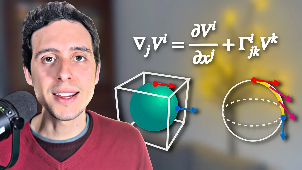
Covariant Differentiation: Learning how to define derivatives on curved manifolds where basis vectors vary from point to point.
Christoffel Symbols and Geodesics: Deriving connection coefficients and solving the geodesic equation to find the shortest paths in curved spacetime.
The Riemann Curvature Tensor: Formulating the mathematical representation of intrinsic curvature and tidal gravity forces.
Einstein's Field Equations: Combining the metric tensor and curvature tensors to describe how mass-energy curves the geometry of spacetime.
26.7K views0likes11:12Original Release: 2011-12-24
welcome to this ongoing series on the theory of relativity in this video we want to investigate the topic of differential geometry a subject of mathematics that plays a central role in our theory I'll try to take a visual approach as much as possible still math is the language of physics and no explanation of relativity is complete without it there's no need to follow the math in any detail but if you are interested more details are given in the appendix videos that are listed in the description box our story begins with carl friedrich gauss fellow who was immensely influential in several areas of math and science in 1818 he was involved in an extensive survey of the german state of hanover and this contributed to his interest in the study of curved surfaces what we now call differential geometry suppose that you're the Royal Road builder and there are a couple of villages that you can toll the bill the road between and the roads supposed to be as short as possible where do you put it I mean it's not as simple as drawing a straight line because you've got hills and valleys do you use intuition trial and error well a scientific approach is to develop a mathematical model of the terrain that describes it in terms of coordinates numbers functions and so on then you formulate the path problem is a mathematical equation that you solve to get a mathematical description of the best path although our terrain exists in three-dimensional space it forms a two-dimensional surface consider the surface represented by a topographic contour map position on the map is uniquely specified by two coordinates say y1 and y2 typically longitude and latitude the third coordinate y3 is represented by labeled cost and elevation contours where the contours are close together the terrain is steep where they are far apart the ground is relatively flat we say this curve two-dimensional surface is quote embedded in flat three-dimensional space it's two-dimensional because each point on the surface is uniquely specified by two numbers y1 and y2 of course the y3 coordinate will have important physical consequences back in the real world consider the road building problem again it might be tempting to say that the shortest path between two points is a straight line so there is a road but one look at the elevation contours and we see that this would take us over a P probably not the shortest path no the shortest path will probably be a curve that avoids the peak and this is analogous to the picture that general relativity paints of particle motion in the presence of a gravitational field in an inertial frame flat space-time particles move along straight lines at constant velocity but when gravity is present curved space-time particles move along curves as dictated by what we might think of as a type of space-time equivalent to elevation contours in both cases were just taking the shortest path between two points we're going to develop our surface model using length measurements and relating those to position on the surface as denoted by coordinate values to get started imagine we have a rectangular graph paper type coordinate system with 1-yard spacing between coordinate lines an arbitrary displacement can be thought of as a displacement in the Y one direction followed by a displacement in the Y two direction then the net displacement s forms the hypotenuse of a right triangle and we can use the Pythagorean theorem to calculate it s squared is equal to y1 squared plus y2 squared so the Pythagorean theorem is the basic tool that allows us to interpret coordinate changes as the distance between two points on the surface now we've seen in previous videos that a graph paper coordinate system won't fit on a curved surface so we've got to consider more general types of coordinate systems to start assume we have rectangular coordinates but the coordinates are not measured in yards we still want to calculate the displacement s in yards so say the chord and x1 is measured in fathoms the Pythagorean theorem only works if the sides of the triangle are all measured in the same units so we're going to need a scale factor a 1 equals 2 yards per fathom then a coordinate change x1 corresponds to a distance a 1x1 yards and suppose the other chord in x2 is measured in feet then we'll need a scale factor a 2 is equal to 1/3 yard per foot and a coordinate change x2 will correspond to a distance a 2x2 yards now we can use the Pythagorean theorem to calculate s squared in yards squared is equal to a 1 squared x1 squared plus a 2 squared x2 squared these scale factors we have to employ called metric coefficients and they will play a central role in everything that follows another thing that could happen is that the coordinate axes are not at right angles these are called non orthogonal coordinates suppose the angle between the axes is Theta and we've used the scale factors a1 and a2 as before so that the sides of the triangle are all measured yards the Pythagorean theorem only works for right triangles so if theta is not ninety degrees we have to make a right triangle with the green lines shown here now a2 x2 is the hypotenuse of a right triangle and we can use trigonometry to get the lengths of the green sides a 2 X 2 times the sine and cosine of theta finally we have a right triangle with s is the hypotenuse and we can apply the Pythagorean theorem to find s expanding and simplifying the expression we end up with our previous a 1 squared x1 squared plus a 2 squared x2 squared terms plus a new term that contains both scale factors and coordinates and the cosine of the angle theta when theta equals 90 degrees that term goes away cosine of 90 degrees is equal to zero and this reduces to our previous result now for bookkeeping convenience we collect the various factors we've developed into an array called the metric tensor the metric tensor is absolutely at the core of general relativity for example one form of metric tensor describes a black hole and other describes Big Bang cosmology and so on for our two-dimensional surface the metric tensor is a 2 by 2 array or matrix and we use subscripts that denote the elements as G 1 1 G 1 2 G 2 1 and G 2 2 and these represent those a 1 squared a 2 squared and a 1 a 2 cosine theta factors we saw previously it's convenient to break the 2 times a 1 a 2 cosine theta factor into 2 1 times a 1 a 2 cosine theta factors because it'll make all the map more symmetric later on so with this labeling our previous result for s squared can be written as G 1 1 X 1 squared plus G 2 2 X 2 squared plus G 1 2 X 1 X 2 plus G 2 1 X 2 X 1 and this is the Pythagorean theorem generalized two scaled and or tilted coordinates a more compact notation is to use the capital Greek letter Sigma to represent a sum and then we have the sum from I equals one to two sum from J equals 1 to 2 of G I J X I XJ we sequentially substitute 1 & 2 for I and J to get the above expression Einstein said let's just drop the Sigma's and write s squared is equal to G IJ X I XJ with the understanding that anytime you see a subscript say I appear twice you're supposed to sum over all possible values so now we have a very nice compact notation for the generalized Pythagorean theorem finally we have to consider what happens when our coordinate system is curved even the generalized Pythagorean theorem only works on triangles so what we have to do is limit consideration at least at any one time to a very small patch of the surface over which the corner curves are essentially lines rigorously this is only valid for vanishingly small displacements that we'll call differential displacements that's the differential and differential geometry and we'll denote these starting with a D as in DX 1 and DX 2 coordinate changes DX 1 and DX 2 correspond to distances that are represented here by little arrows notice that the same DX 2 change that is from one green line to the next can represent a different length depending on where it occurs on the surface so when we write our generalized Pythagorean theorem now the metric coefficients the scale factors have to be functions of position and notice also that the distance D s here is a differential distance a very very small distance instead of the S squared we had before now we have all the tools we need to figure out distances in terms of any coordinate system on any surface one more visual aid for thinking about our distance formula you can take the 2 by 2 metric tensor and write the differential displacements DX 1 and DX 2 above and to the left and then for each metric coefficient multiplied by the DX value in that row and the DX value in that column and do that for all four coefficients add the results together and you get the generalized Pythagorean theorem what's called the first fundamental form of differential geometry now let's apply all this to our path problem on a curved landscape suppose this surface is a mathematical representation of the landscape in an aerial view we lose the 3d perspective on elevation although we can represent it by elevation contours we want to be able to relate displacement on the map to displacement on the ground suppose we're interested in the black path shown here let's take a cross-sectional slice of the surface and view it in profile we end up with a plot of elevation vertically versus the x1 coordinate from the map horizontally now suppose we go to x1 equals 10 on the map and ask what ground displacement D s results from a map displacement DX 1 in this case the ground is essentially level so D s and D x1 would be essentially the same however if we do the same thing at x1 equals 30 because the surface is sloped there will get a larger DS for the same DX 1 these effects are what the metric coefficients account for at x1 equals 10 G 1 1 is essentially 1 while at x1 equals 30 G 1 1 is something larger than 1 and we can see that as the slope of the ground gets larger the g11 coefficient will have to also in the extreme case that the slope is infinity that would be a sheer cliff G 1 1 would approach infinity in other words if you fall off a cliff you don't change your longitude or latitude so your position on the map won't be changing but you'll still be doing a whole lot of moving it'll just all be in the downward direction in fact we'll see that this is one way to view what happens at the event horizon of a black hole there are one of the space-time metric coefficients goes to infinity and the interpretation is that someone approaching the horizon would perceive herself to be moving rapidly while a distant observer would not see her moving at all so now if we know the metric coefficients at all points on the map we can take any path say the black curve shown here and go along at adding up all the DS displacements on the ground corresponding to our dx1 dx2 displacements on the map and arrive at the total on-the-ground length of the path is then possible in principle to solve for the shortest possible path between any two points so we've looked at some examples of the way differential geometry was developed and how it can be applied to analyze surfaces in the next video we'll see how other mathematicians extended Gauss's work from two-dimensional surfaces into abstract n dimensional spaces and how this provided an ideal mathematical framework for the physical einstein had developed
Up Next
7:42
Understanding Gaussian Curvature Through Pizza: A Mathematical Insight
@numberphile
1.5M views•2016-06-16

4:43
Elliptic Curve Cryptography Explained: ECC, ECDSA, ECDH
@PracticalNetworking
28.5K views•2024-10-21

10:44
Fourier Series Introduction: The Big Idea Explained
@DrTrefor
387K views•2021-05-03

6:00
The Mathematical Impossibility of Accurate World Maps
@Vox
23.3M views•2016-12-02
Related Study Plans & Knowledge Roadmaps
Structured learning paths in Mathematics
mathematics
Tensor Calculus: Vectors to Riemann Curvature
01Mathematical Foundations: Linear Algebra & Calculus
02Covectors, Dual Spaces, and Tensor Basics
03The Metric Tensor and Index Gymnastics
+ 2 more learning modules
40h5 modules
Explore Roadmap
mathematics
Gödel's Incompleteness: Logic, Proofs & Limits
01Introduction to Formal Systems & Hilbert's Dream
02Set Theory, Cardinality, and Cantor's Diagonal Argument
03Arithmetization and Gödel Numbering
+ 2 more learning modules
14h5 modules
Explore Roadmap
mathematics
Galois Theory: Fields, Groups & Solvability
01Foundations of Abstract Algebra: Groups & Fields
02Polynomials & Field Extensions
03Splitting Fields & Symmetries
+ 2 more learning modules
24h5 modules
Explore Roadmap
mathematics
Non-Euclidean Geometry: Models & Geodesics
01Euclid's Fifth Postulate and the Birth of New Geometries
02Hyperbolic Space and the Poincaré Disk Model
03Geodesics: Defining Straight Lines in Curved Spaces
+ 2 more learning modules
15h5 modules
Explore Roadmap