














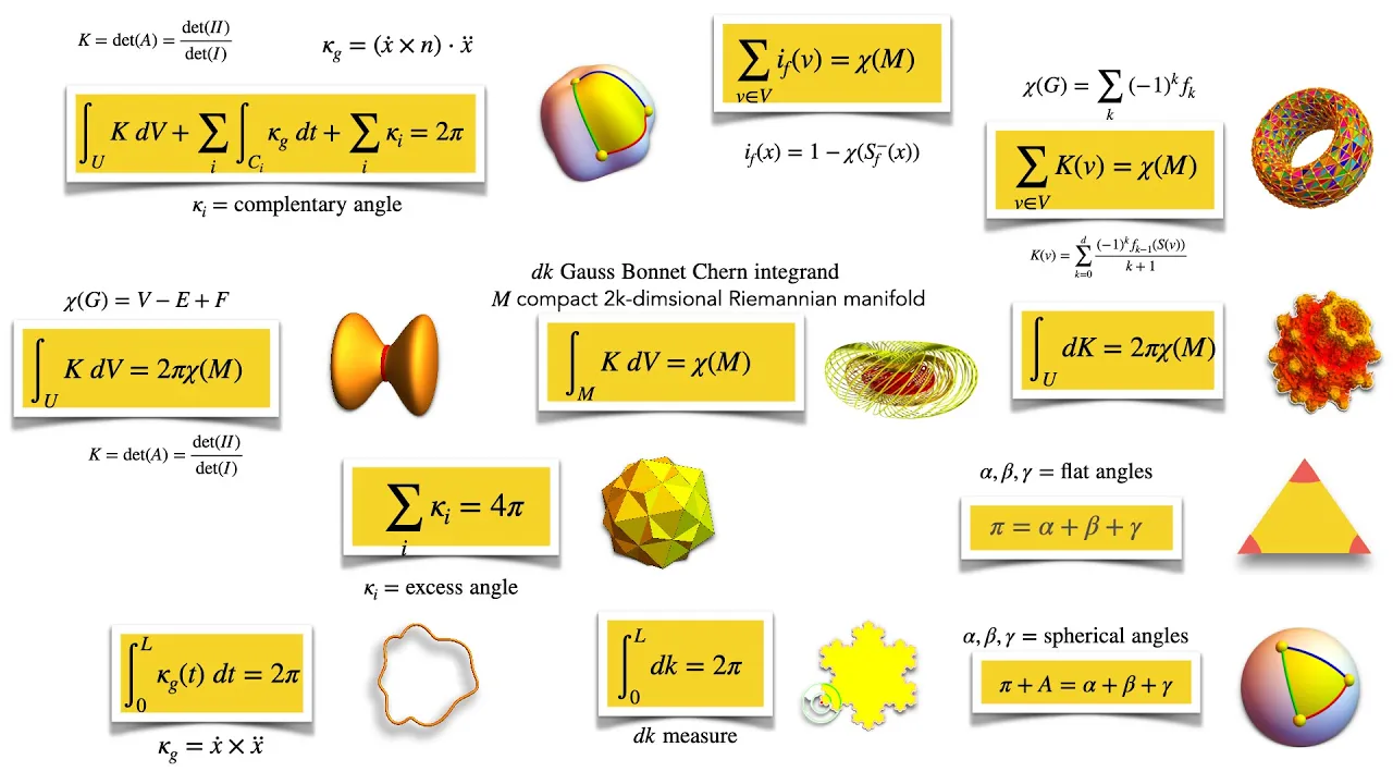
The Gauss-Bonnet Theorem states that for a simple closed smooth curve on a surface, the line integral of the geodesic curvature equals 2π minus the surface integral of the Gaussian curvature over the interior region, mathematically expressed as ∫γ kg ds = 2π - ∫∫D K dσ, where kg is the geodesic curvature, K is the Gaussian curvature, and D is the region enclosed by the curve γ.
Gauss-Bonnet Theorem for Simple Smooth Curves | Differential Geometry
Added:Fundamental concepts of curves on surfaces, specifically the definition and geometric meaning of geodesic curvature.
An understanding of Gaussian curvature of a surface and how it is calculated using the first and second fundamental forms.
Proficiency with vector calculus theorems, particularly Green's Theorem and Stokes' Theorem, which are used to relate line integrals to surface integrals.
Familiarity with the concept of the covariant derivative and frame fields (such as Cartan's moving frames) on a surface.
The Global Gauss-Bonnet Theorem, which links the total Gaussian curvature of a compact surface to its topological Euler characteristic.
Generalizing the theorem to piecewise smooth curves (curves with corners), which introduces the concept of exterior angles.
Applications to non-Euclidean geometry, such as calculating the area of geodesic triangles on spheres and hyperbolic planes.
An introduction to Chern-Weil theory and the generalized Gauss-Bonnet-Chern theorem in higher-dimensional Riemannian geometry.
735 views18likes12:30Original Release: 2025-02-13
hello students in this video we'll prove the gaus banet theorem for simple closed curves let's let U of T V of T be a simple closed curve just looking c three on AB so that just means if I look at this curve and plug in the initial point and plug in the terminal point the initial point and terminal point have to be the same there's our curve we can call this curve over here gamma for example I'll just leave like that for time being looks like this there's no there's no jumps so in other words both these functions are infinitely differentiable so we can assume that u and v are infinitely differentiable and so no words there's no cusps over here I don't have a situation where there's going to be a point where the derivative doesn't exist just nice simple curve right and let R be a surface parameterization like that beautiful then gamma T which is R of U of TV f is a closed curve on the surface okay so here's your surface right like that and then the image under this parameterization of this curve gives you some curve like that right so this is your curve gamma over here okay and now what does the gaus B theorem say the gaus b theorem says in this case that if I integrate over the curve gamma the geodesic curvature that is 2 pi minus the double integral over the interior of gamma of the gausian curvature with respect to the surface area differential okay beautiful that's a wonderful theorem that relates the global curvature right on the on the interior of the curve to the gesc curvature on the boundary okay and so here's we're going to do we're going to let FG be an orthonormal basis of the tangent space to the surface at every Point okay there I set before so I've choose an orthal basis I can do this by Gram we already know properties of this orthonormal basis right then if Theta of s is the angle between F at and Gamma dot then gamma dot is going to be F I'm going to suppress the uh of s here right just cosine of theta plus Gat sin Theta because it's an orthonormal basis I can write down this expression and then this implies that the component n cross gamma dot has to be what has to be F negative f sin theta plus Gat cosine Theta okay beautiful and now of course here comes the the second der has to pop up because I know if I take this expression over here and Dot this with gamma double dot that gives me the G curvature so let's do that so what's gamma double dot going to be so here's the tricky part so gamma double dot is going to be F do cosine theta plus g dot g do sin Theta then minus F cosine Theta Theta Dot and then plus G hat cosine Theta oh I have to do the D so that's going to be a sign of course right because der of cosine is s so it's going to be an F hat sin Theta th dot plus G hat cosine Theta Theta dot okay so what's my Kappa G going to be so let's do it slowly so my Kappa G is going to be what cap G is going to be well let's do this over here so we're going to have a now what do we know so here's an elementary observation so what can I say about I know that fat. Gat is equal to zero because it's an orthal basis and I also know F any derivative of f f hat dot do fat is equal to zero and G hat dot do G hat is also equal to zero because they're unit vectors right good all right so those are things that we're going to use in our calculation over here so if I do for example if I do this term over here do this term it's zero because F hat dot f hat. fat dot is zero so these first terms is give me a what an F hat dot g hat dot g hat cosine 2 Theta so the dot over there goes on the F then what do we do next then I got to do this term so this dot the G will be zero because of unit Vector so I'm going to get a minus F hat G hat Dot sin^2 Theta good and then that takes care of these terms over here right then if I have F and then F that gives me a one by unit Vector so that's going to be a just a sin squ Theta dot plus sin s Theta Theta Dot and then f.g is equal to Zer by orth orthogonality g. f is equal to zero and then g. G is equal to 1 so this going to be a plus cosine 2 Theta Theta dot right I'm going to do one thing over here I'm going to take this derivative over here on the F Dot and pass it to the g dot so all total the GS curvature is going to give me what the GS of curvature these terms just to add up to Theta dot so I get a Theta dot over here and then we have minus fat G hat dot right and then if I do that or if I put the dot over here that's a negative cosine Square Theta negative sin Square Theta gives just a negative one over here beautiful right and so now what do we know I'm going to write down what G hat is going to be right on this curve this is going to be Theta dot minus fat and then we're going to have a gat u u dot plus G hat V V Dot like that okay so that's a little bit of a nicer expression now let me integrate this okay so if I integrate kg that's the same as integrating this over here so the integral over gamma of the gsit curvature DS is going to be well if I integrate Theta dot that's a perfect derivative integrating Theta dot around the closed curve gives me 2 pi okay now that's actually I'm sweeping something important under the rug over here what I'm sweeping over here is the fact that Theta integrates over the unit circle to that that the integral over gamma Theta dot DS is equal to 2 pi this is an important relationship it's true for any simple close curve and that's known as the H lat and we won't prove that in this video because it requires homotopy Theory so we need a little bit of homotopy theory in order to prove this theorem but you can think about what happens in the case of like a circle for example if if you measure how much the the angle is changing as you Traverse the unit circle the it changes by 2 pi right that's how much the circle changes now of course you can sort of think if I deform the circle a little bit so there's the the case of the circle is easy but if I just deform the circle to some other sort of strange curve like this well in that cas case it's basically still encapsulated I can basically take that more strange curve and continuously deform it onto the unit circle so if there's a that's what a homotopy is right so in other words if I can if two curves are homotopic then I know they're going to show the same index or the same winding number right so that requires a little more work but intuitively it should be obvious that gives us 2 pi okay good and then minus this thing over here F hat and then gu U du that's a u and then a plus f g v DV like so DS okay get R the DS now it's just a regular line integral right I just put the different I write the DS as a line integral now okay and now of course I can t of green St and you you should have expected green St because it's the interior of gamma over here right so let me use green STM so is going to be 2 piun minus the double integral over the interior of gamma and then I got to do the what I got to do the U derivative of this and then minus the V derivative of the first thing the V derivative of this thing over here f g U and that's going to be a DA okay not a d Sigma right but what do we know about this when we do when we do this product I'm going to have an F UV then I'm going to have an F then I'm have an FG V and over here I'll have an F gvu so the G the when the derivatives go on the GV or when the Der goes on the GU those terms are going to cancel and you'll just have an f u v minus fvg so these terms over here are going to work out to be what those to f u g v minus f v g u and we have from our previous LMA that that's exactly equal to what that's exactly equal to the Ln minus m^2 over the square root of EG so that this whole thing was going to simplify to what this whole thing just simplifies to 2 pi minus a double integral over the interior of gamma and and then just the gausian curvature k d Sigma and what we're really using here is we're using what fact we're using the fact that this this quantity over here is equal to l Ln - m^ 2 over the < TK of EEG - f^ s right we have that from a previous video now of course that's not K but if I put it in extra Factor EG - f^2 over EG - f^2 then this this expression over here is the what that expression is the gausian curvature because now it has the right form and what's left over adjust the area differential into the surface area differential and that proves the first version of the gaus banet theorem which says that if I integrate the G of curvature over the curve that's 2 pi minus the gausian curvature over the interior of that curve beautiful result in further videos we'll extend this to the case when you don't have a smooth curve you have cusps on your curve and that basically introduces more angles into the problem thank you very much much
Up Next

55:55
Gauss Bonnet Theorem Proof | Differential Geometry Lecture 27
@jamescook5617
7.9K views•2015-08-07

4:43
Elliptic Curve Cryptography Explained: ECC, ECDSA, ECDH
@PracticalNetworking
28.5K views•2024-10-21

10:57
Geodesics Defined: Zero Curvature & Deriving Geodesic Equations
@mikethemathematician
501 views•2025-01-25

6:00
The Mathematical Impossibility of Accurate World Maps
@Vox
23.3M views•2016-12-02
Related Study Plans & Knowledge Roadmaps
Structured learning paths in Mathematics
mathematics
Tensor Calculus: Vectors to Riemann Curvature
01Mathematical Foundations: Linear Algebra & Calculus
02Covectors, Dual Spaces, and Tensor Basics
03The Metric Tensor and Index Gymnastics
+ 2 more learning modules
40h5 modules
Explore Roadmap
mathematics
Gödel's Incompleteness: Logic, Proofs & Limits
01Introduction to Formal Systems & Hilbert's Dream
02Set Theory, Cardinality, and Cantor's Diagonal Argument
03Arithmetization and Gödel Numbering
+ 2 more learning modules
14h5 modules
Explore Roadmap
mathematics
Galois Theory: Fields, Groups & Solvability
01Foundations of Abstract Algebra: Groups & Fields
02Polynomials & Field Extensions
03Splitting Fields & Symmetries
+ 2 more learning modules
24h5 modules
Explore Roadmap
mathematics
Non-Euclidean Geometry: Models & Geodesics
01Euclid's Fifth Postulate and the Birth of New Geometries
02Hyperbolic Space and the Poincaré Disk Model
03Geodesics: Defining Straight Lines in Curved Spaces
+ 2 more learning modules
15h5 modules
Explore Roadmap