![CAP5415 Lecture 6 [Introduction to Convolutional Neural Networks - Part 1] - Fall 2020](https://i.ytimg.com/vi/GwMxGEFjF5E/hqdefault.jpg)
![[TensorFlow 2.x 강의 13] 합성곱 신경망 CNN 기초](https://i.ytimg.com/vi/1_70qe1XBV8/maxresdefault.jpg)
![[Mì Python] Bài 5. Python với Keras và CNN (Phần 2/2)](https://i.ytimg.com/vi/gv693bG9K98/maxresdefault.jpg)


![[컴퓨터비전 2026] Lecture 13. Image Segmentation](https://i.ytimg.com/vi/ZHn6iPH1nhU/maxresdefault.jpg)





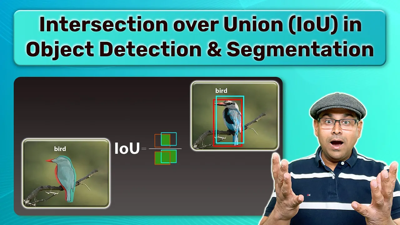





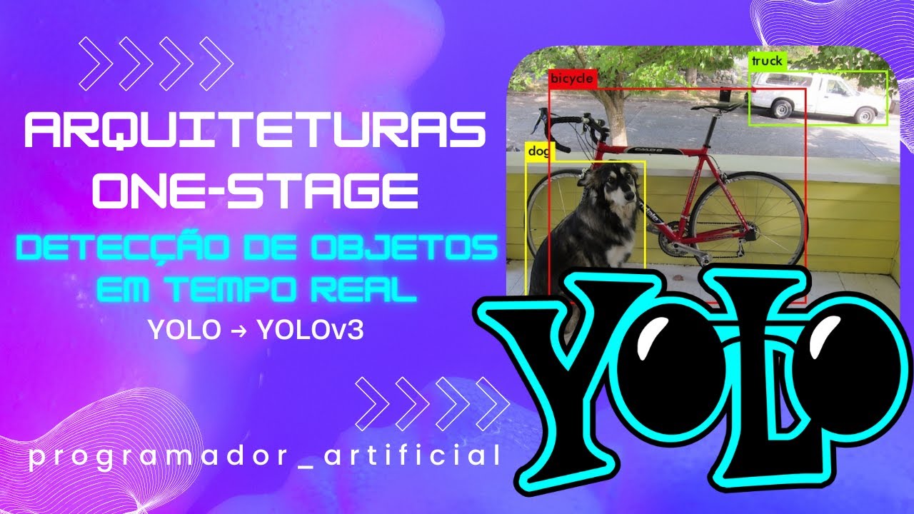






YOLO (You Only Look Once) is a real-time object detection framework that processes an image in a single pass using a single convolutional neural network, dividing the input image into a grid where each cell predicts multiple bounding boxes with associated confidence scores and class probabilities, then combining this information through a loss function that includes class loss, localization loss, and confidence loss to achieve fast and efficient object detection while maintaining reasonable accuracy.
YOLO Object Detection Explained: Algorithm and Architecture
Added:Fundamentals of Convolutional Neural Networks (CNNs), including convolution operations, pooling layers, and feature map extraction.
The core difference between Image Classification (predicting 'what') and Object Detection (predicting 'what' and 'where').
Basic mathematical understanding of regression and classification loss functions, such as Mean Squared Error and Cross-Entropy.
The concept of Intersection over Union (IoU) as a metric to evaluate the overlap between predicted and ground-truth bounding boxes.
The evolution of the YOLO architecture through successive versions (from YOLOv2 to the latest YOLOv8 and beyond), detailing how features like anchor boxes and feature pyramid networks were integrated.
A comparative study of One-Stage detectors (YOLO, SSD) versus Two-Stage detectors (Faster R-CNN) to understand trade-offs between inference speed and detection accuracy.
Evaluation metrics specific to object detection, primarily Mean Average Precision (mAP) at different IoU thresholds.
Hands-on implementation and transfer learning using YOLO on custom datasets, followed by model optimization for edge deployment using TensorRT or ONNX.
134.4K views2.9Klikes17:04Original Release: 2023-03-12
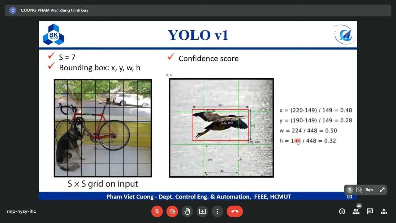
hello so today I'm going to be talking about YOLO which is a highly influential algorithm and framework used for real-time object detection which means it has a very wide range of applications including video surveillance uh self-driving cars face detection during during the pandemic to measure temperatures and that kind of thing so it's uh in in short it's it's a very popular algorithm that's been used a lot in the past several years and the goal here is simply to create bounding boxes around the objects in an image and then also to label these objects according to their class now these sorts of object detection methods have been around for several years but YOLO and its variants seem to capture a desirable mix between speed and accuracy now the actual definition of mean average Precision is a bit more subtle than that but let's not worry about that for now so as you can see out of the models that are capable of what we can call real-time detection or into their speed YOLO seems to deliver the best performance despite still being less accurate than some of the slower models and the reason YOLO is able to achieve this is that it utilizes powerful deep learning architecture while at the same time using the input image data in a highly efficient way so just to compare with some prior developed models the deformable parts model or DPM uses filters that represent whole objects and parts of objects to create a detection confidence map using a sliding window technique and the idea here is that an object is likely present if all of its parts are present even if they are configured in unusual ways now region-based cnns do kind of the same task but differently here you have three separate models a region proposal Model A CNN that that extracts a feature vector and then a support Vector machine for each class now these three models notably are typically trained separately and even though there have been many developments on the RNN approach since 2014 the essential idea of region proposal plus classification still applies now the distinguishing feature of YOLO is that instead of looking at an image multiple times whether it's to apply the deformable parts filters or to inspect the regions like the rcnn you only look at the image once so just to summarize how this scheme works the first step is to overlay on an input image a grid with s grid cells on each axis each grid cell then produces two things one it produces a set of bounding boxes centered on a point inside the grid cell with Associated confidence scores that an object exists inside each bounding box and then it also produces a class probability map for each grid cell which essentially tells what object class is most likely to be in that cell given that an object in fact exists in the Cell at all and finally it combines this information to yield the object detections so that's the abstracted framework but how does it actually work in practice well for each grid cell we compute a set of output vectors the first Vector is a vector of class probabilities the second is a set of bounding box parameters specifying the X and Y position of the center of the bounding box as well as the square root of the width and the height of the box and I'll explain why we take the square root a bit later and then finally we also have the confidence score denoting the model's confidence that an object in fact exists in the Box now instead of having just one bounding box each grid cell will typically have multiple boxes and this just allows the cell to detect more than one object now in practice instead of having several vectors we just combine them into one big Vector with length B times 5 plus n where n is the number of object classes now B is the number of bounding boxes per grid cell and in the original paper the authors use a seven by seven grid with two bounding boxes per cell and 20 classes so for each grid cell we output a length 30 vector but how exactly does this model just go from an input image to these output vectors well simply we just use a CNN on a convolutional neural network now this architecture just consists of a stack of convolutional layers that distill an image into a more abstract representation followed by two fully connected layers that transform this into an output Vector for each grid cell and there's three channels in the input just represent the red green and blue channels in the image cool so now that we have an idea of how the model Works let's look at how it is trained let's say we are trying to predict uh say this bounding box now the center of the batting box is at this point here so this grid cell will be responsible for it well let's say we've predicted this green box here along with the five parameters that Define it X Y location the width the height and the confidence and we want to somehow penalize the prediction because it isn't exactly the same as the ground truth but what would the grand truth values be well for the class probabilities this is simply one for the correct class and zero for everything else note that this assumes that the classes are mutually exclusive and with later versions of YOLO I think starting with yellow version three the model is actually capable of multi-label classification where two classes can exist simultaneously such as dog and animal um but YOLO V1 just predicts one class so that's cool now let's see how we calculate the coordinates of the ground truth and predicted boxes well X and Y are usually calculated with respect to the top left corner of each individual grid cell and they are also expressed as a proportion of the total grid cell dimensions meanwhile the widths and the height are expressed as a proportion of the Total Image dimensions hence these all fall into the zero to one range so just to take a quick example let's say that the coordinates of the point are 16 and 44 pixels respectively from the top left origin of the entire image let's say each grid cell is 10 by 10 pixels and the image has seven grid cells on each axis then the X and Y values are 0.6 and 0.4 respectively or the percentage sign here is just the modulo operator and the width and the height are obtained by dividing by 70.
um yeah well so what about the confidence well essentially with confidence the question we're asking is does an object appear in the grid cell or not and confidence is the score attached to the positive answer the third question so let's say that we have these ground truths bounding boxes with these Center points and these good cells responsible then in every grid cell except for those grid cells the ground truth confidence is set to zero because there isn't an object there meanwhile in the green grid cells the ground truth confidence is simply the intersection over Union of the predicted and ground truth bounding boxes just to review what intersection of reunion means uh the intersection between two sets or two boxes in this case is the area of the shared region so it's the middle figure here while the union is the combined area of both of the boxes without double counting the overlap so the intersection of reunion of A and B is then simply the intersection divided by the Union that's essentially a measure of the degree of overlap between two boxes or sets more generally so the ground truth confidence is simply the IOU of the predicted and ground boxes however we know that each grid cell can produce multiple predicted boxes so which one should we choose well during training in order to calculate the loss we just use the predicted box that is the highest IOU with the true box incidentally the authors of the original paper note that by assigning only one predicted box to each ground truth box the different predictors are able to specialize and perform better on certain object classes or aspect ratios or whatever now similarly during inference if we have two predictions P1 and P2 then if the IOU between them is greater than some threshold we only keep the one that is associated with the higher confidence in the presence of an object now this whole process called non-max suppression just trimmed down the predicted boxes to prevent any overlaps between them so now that we know how all of the Box prowders are calculated let's see how they are used in the loss function now the total loss function is basically just a sum of two terms and the object class loss which operates on the class probabilities and the localization loss which operates on the bounded box parameters and this is what the class loss looks like so instead of using a cross entropy or anything like that we just take the sum squared error between the predicted and ground truth class probabilities summed over all classes and all grid cells now this uh interesting symbol here just means that we're only considering the class loss of a grid cell I If an object in fact exists within that grid cell um so recall the probability map that I showed earlier there here there are plenty of cases where the model has project has predicted an object class where it's actually a background and we're actually not counting those cases in the class loss the class loss only deals with cases where an object has been mistaken for another object and not where there is in fact a background so what about the localization loss well this is also split into a confidence loss and a box coordinate loss the coordinate loss is summed over all grid cells and all bounding boxes in each grid cell but it is only counted for those cases where cell I contains an object and box J is deemed responsible for that object so here we sum the squared error of the X and Y coordinates as well as the square root of the width and height we also scale this entire thing according to a parameter Lambda chord and I'll explain why this happens in a bit now the confidence loss has a very similar form except that the grid cells which do not contain an object are scaled by a parameter Lambda No Object while those that do in fact contain an object are not scaled and again I'll explain why this happens in a bit so here is the entire loss function what's apparent is that we're just using squared error to obtain good values for the class probabilities and all of the bounding box parameters so in this sense object detection is just reduced to a regression problem and this gives YOLO a sense of simplicity so it really is just regressing all of these values here without anything fancy like you know cross entropy losses or anything like that so uh from this we know that YOLO works very well but what are some of its limitations uh and here I'm talking more specifically about the first version of YOLO well first of all of course each cell can only contain one class so if or it can only predict one class should I say um so if say one dog and one bicycle appear in the same grid cell then this presents a problem moreover each grid cell contains a finite specified number of bounding boxes so if there are many objects appear in one grid cell then this also presents a problem one example is busy Urban environments where there might be you know multiple people in each grid cell now the authors note some other limitations which include the fact that Banning box predictions tends to struggle with unusual aspect ratios or configurations of object that it had not sufficiently seen in the training data and furthermore the loss function deals with only with absolute values of x y w and H so it cannot deal with the fact that the same absolute error will matter more in a small box than in a large box there is no explicit error scaling according to the size of the bounding boxes but one method the authors developed to tackle this is to use the square root of the width and the height rather than just the width and the height and this means that as the box size scales linearly the square root of w and H scale sublinearly which in effect suppresses differences between large and small boxes and now the final consideration is that many cells do not in fact contain an image and the consequences of this are twofold in training the confidence scores are liable to be pushed to zero since this is the ground Truth for most of the cells in an image and furthermore since the coordinate loss is calculated only for cells with objects it will tend to be underrepresented in the final loss so in order to address both of these problems we can scale the No Object confidence scores we can scale down the No Object confidence scores and scale up the coordinate losses using the Lambda scaling factors and in the original paper the authors set Lambda No Object to 0.5 and Lambda chord uh to five so there we have it YOLO is a fast and effective object detection framework that works because of its Simplicity using just a single CNN to learn the bounding boxes and class identities of each object in an image now the yellow scheme I've introduced here was developed way back in 2015-16 and since then many other versions and improvements have come out so if you're interested please take a look at them but for now thanks for watching
Up Next

42:30
Training YOLOv8 on Custom Datasets for Object Detection | Step-by-Step Tutorial
@dswithbappy
169.3K views•2023-01-28

87:26
Introduction to Secure Multiparty Computation with Yehuda Lindell
@fhe_org
7.7K views•2021-02-04

4:55
HTTP Requests Explained: GET, POST, PUT, DELETE
@codecademy
103.1K views•2021-10-07

19:25
Enigma Machine Mechanics: WWII Encryption Explained
@JaredOwen
13.2M views•2021-12-11
Related Study Plans & Knowledge Roadmaps
Structured learning paths in Computer Science
computer-science
Container Runtimes: Namespaces, Cgroups & Go
01Linux Systems & Go Programming Foundations
02The Core of Isolation: Chroot and Filesystems
03Linux Namespaces: Process Isolation
+ 3 more learning modules
32h6 modules
Explore Roadmap
computer-science
Building a CHIP-8 Emulator: Rust & CPU Basics
01Computer Architecture Foundations (Bits & Bytes)
02Rust Programming for Systems Development
03CHIP-8 Virtual Hardware Specifications
+ 2 more learning modules
32h5 modules
Explore Roadmap
computer-science
Building BitTorrent: Go, P2P & Concurrency
01Go Fundamentals & Concurrency
02Networking Foundations & P2P Architecture
03Bencode Parsing & Torrent Metadata
+ 3 more learning modules
26h6 modules
Explore Roadmap
computer-science
Actor Models (C++ Concurrency & Lock-Free)
01C++ Multi-Threading Foundations
02Thread Pools and Task Scheduling
03Atomics and Lock-Free Queue Design
+ 3 more learning modules
45h6 modules
Explore Roadmap