









![[확률미분방정식] 확률미분방정식의 기호 정리 , Stochastic Differential Equations](https://i.ytimg.com/vi/Qk_mwvnJ8_U/hqdefault.jpg?sqp=-oaymwEmCOADEOgC8quKqQMa8AEB-AH-CYAC0AWKAgwIABABGGUgZShlMA8=&rs=AOn4CLCVdRZxlOWc6Y--IXwN5nJ7zcADRA)










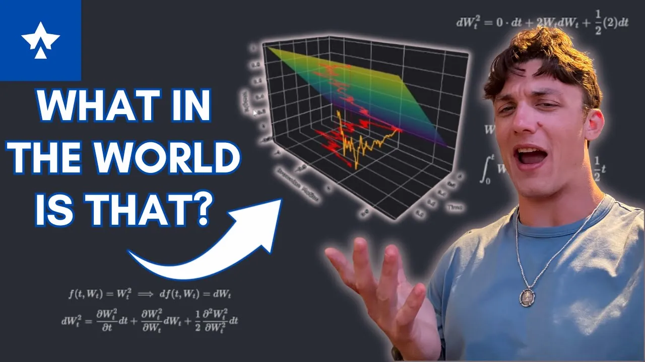
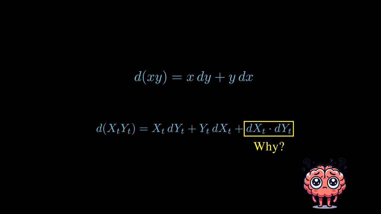
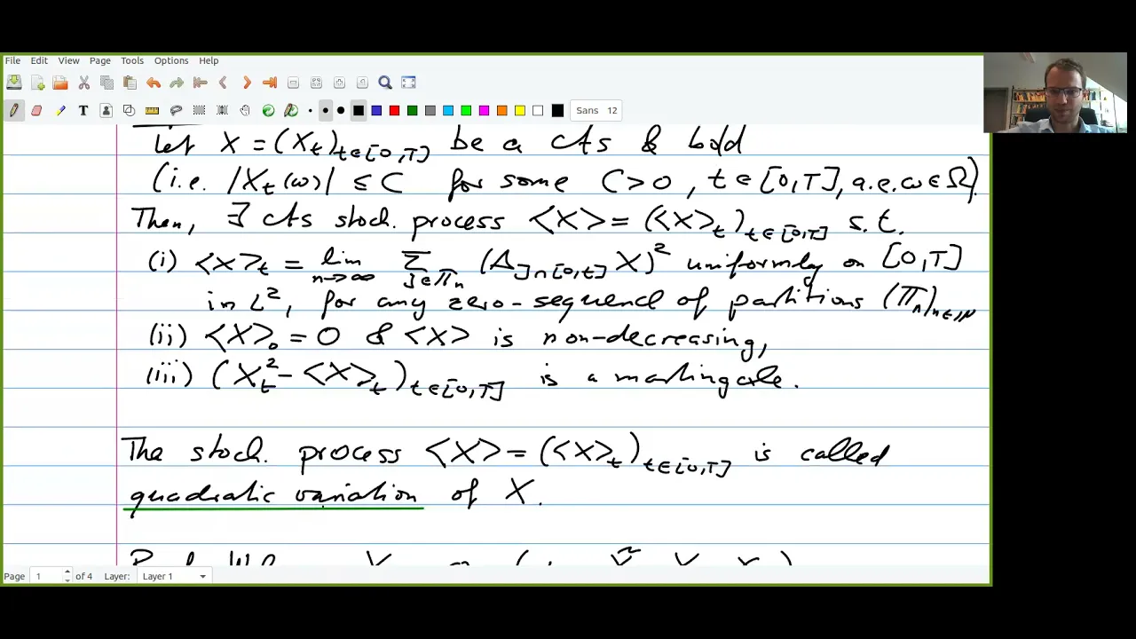
Ito's lemma is the stochastic equivalent of the chain rule in ordinary calculus, which states that for a function f(X_t, t) of a stochastic process X_t driven by Brownian motion, the differential df = (∂f/∂t)dt + (∂f/∂x)dX_t + (1/2)(∂²f/∂x²)(dX_t)², where the extra (1/2)(∂²f/∂x²)(dX_t)² term arises from the non-zero quadratic variation of Brownian motion. The proof involves dividing the interval into subintervals, applying Taylor expansion, and showing that the second-order term converges to the integral form using mean square convergence and iterated expectation properties.
Ito's Lemma Derivation: Stochastic Chain Rule Proof | Step-by-Step
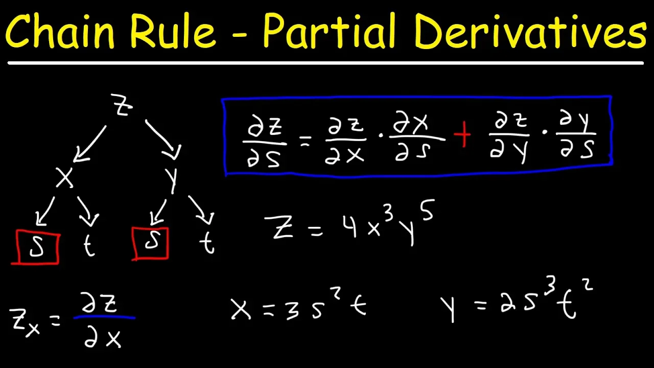
Added:Standard Calculus Chain Rule and Multivariable Taylor Series Expansion: Understanding how to expand functions of multiple variables up to the second order.
Properties of Brownian Motion (Wiener Process): Familiarity with its continuous but non-differentiable paths and the heuristic scaling behavior of its increments.
Concept of Quadratic Variation: Knowing how quadratic variation is defined for stochastic processes and why it does not vanish for Brownian motion.
Basic Stochastic Differential Equations (SDE) Notation: Comfort with the informal differential notation used in stochastic calculus (e.g., dX_t).
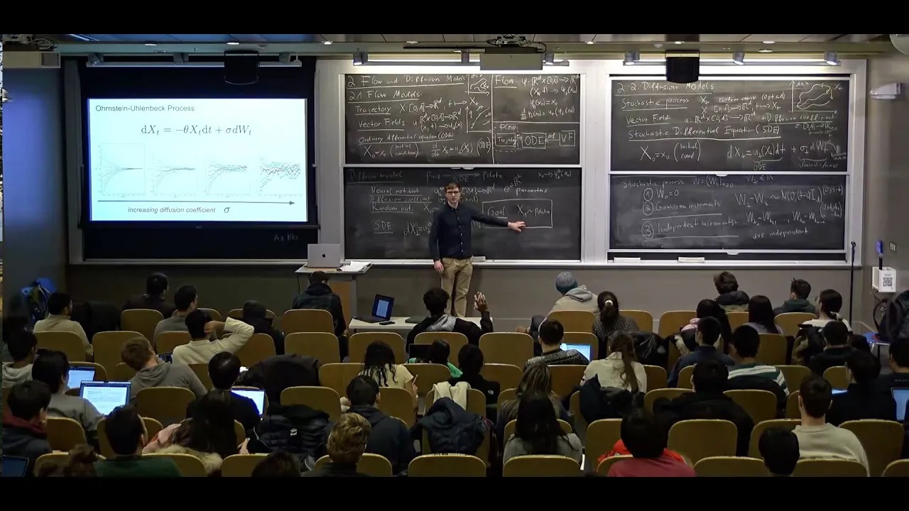
Solving Stochastic Differential Equations (SDEs): Applying Ito's Lemma to find explicit solutions for processes like Geometric Brownian Motion and the Ornstein-Uhlenbeck process.
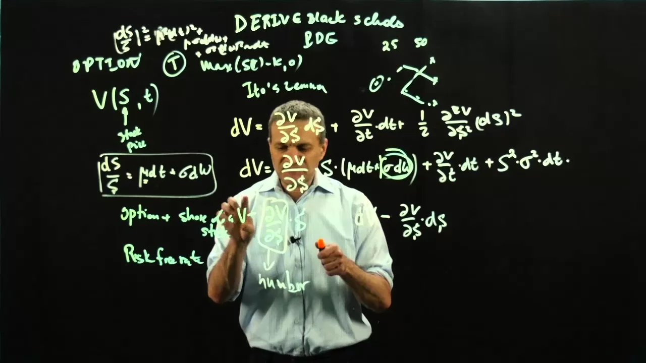
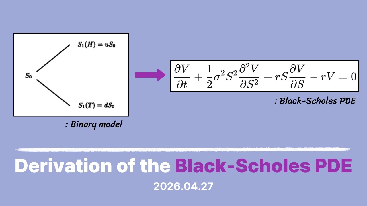
Derivation of the Black-Scholes PDE: Using Ito's Lemma to model asset price dynamics and derive the fundamental partial differential equation for option pricing.
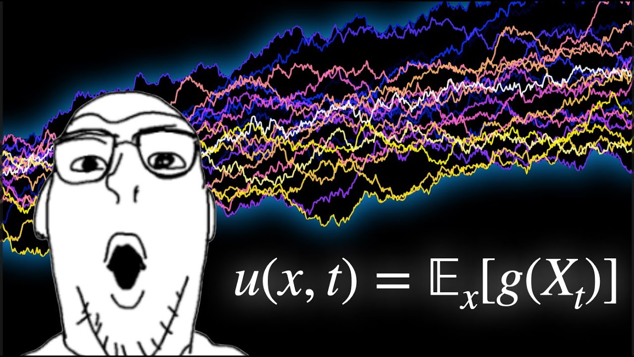
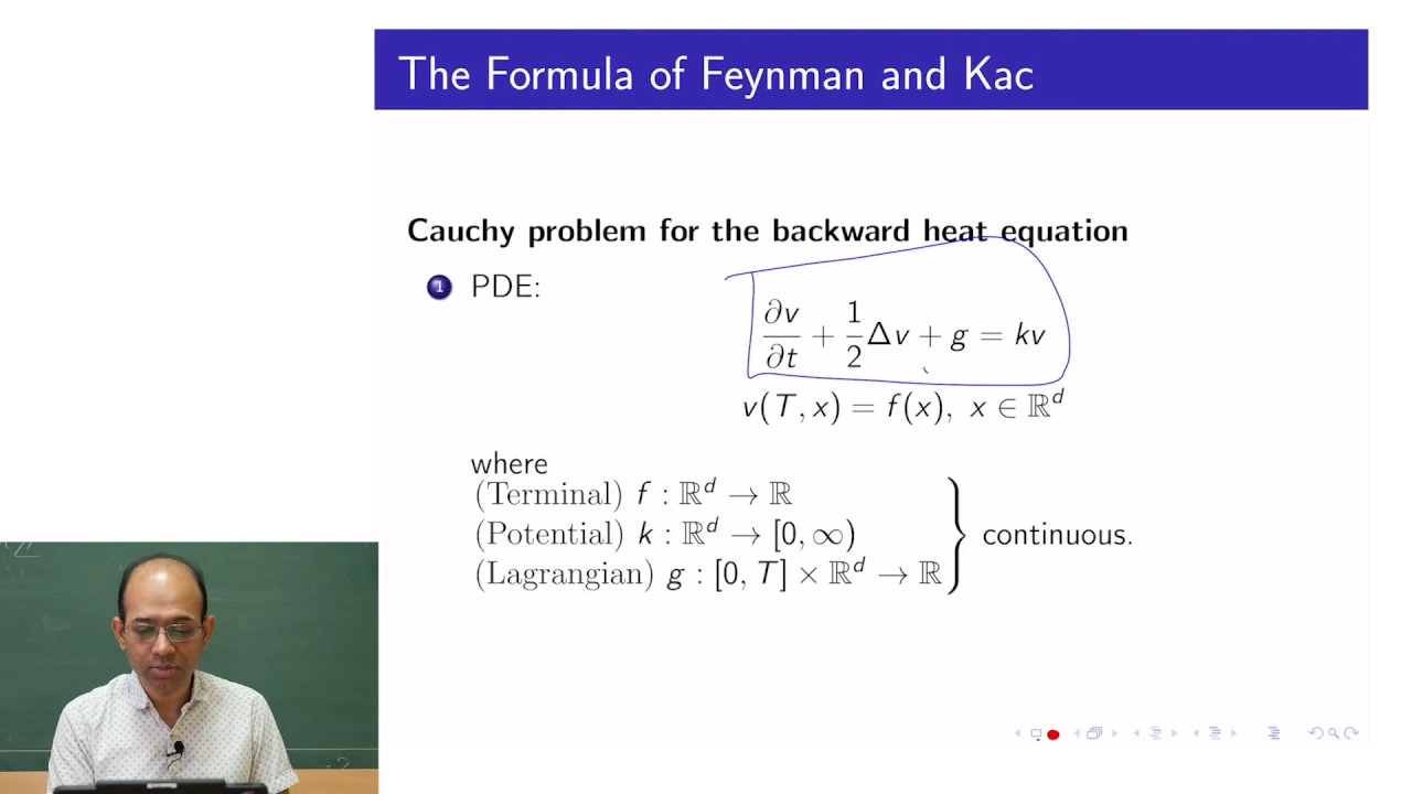
The Feynman-Kac Theorem: Exploring the mathematical bridge between stochastic differential equations and deterministic partial differential equations.
Multidimensional Ito's Lemma: Extending the stochastic chain rule to systems with multiple, correlated stochastic processes.
25.4K views259likes11:27Original Release: 2018-12-09
hello and welcome to quantify in this video we are going to derive the Ito's lemma which is the stochastic equivalent of the chain rule of calculus this formula applies when the Ito's interpretation of stochastic integration is assumed recall from calculus that if Y is a function of U then the differential of Y is defined as follows now if a stochastic process X is a function of Brownian motion then its differential is defined as follows for the purists we have implicitly assumed that the function is twice continuously differentiable and this assumption will become explicit when we get to the proof comparing the deterministic and the stochastic chain rules we see that the stochastic version has an extra term the stochastic chain rule is known as Ito's lemma it is also commonly referred to as Ito's formula we can write it in integral form as follows and if X happened to be a function of T as well then we will need to add one more term to this which is just the partial derivative with respect to t times delta T this result is valid for a much larger class of stochastic processes the so-called semi martingale but we will prove the result using the Brownian motion as an example this is easy to do because we already know the properties of the Brownian motion and its integrals as you would expect extension to semi martingale is only a matter of exposure to this broader class of processes to prove the formula let's write the differential as the difference between the end and the start values of the process as X is function of Brownian we can write it in terms of the function values as follows now let's divide the interval from 0 to t into n subintervals and let's write the overall change as the sum of the changes over the sub intervals this is just the telescoping sum formula in Reverse now recall this formula from calculus notice this is an exact formula and not the truncated Taylor series but you can view this as truncated Taylor series which has been made exact through the mean value theorem notice the derivative is at the left end point whereas the second derivative is somewhere in the interval and is chosen to make the formula exact now in terms of the Brownian increments this formula becomes looks longer and complicated but we just substituted the Brownian motion value at the left end of the interval for a and the Brownian motion value at the right end of the interval for B we also substituted K prime for C so as to make it clear that this point belongs to the case interval substituting listen to the summation formula we get splitting the two components we get now the first term in the limit as n tends to infinity is precisely the definition of Ito's integral the second term is complicated because the point at which the function is evaluated is not at the left end of the interval that the Ito's integration assumes and you can see that in order to prove the Ito's lemma the only thing we need to show is that the second component converges to an integral that we can make sense of and that's exactly what we are going to do now we are going to prove the convergence of the second summation to an integral in two steps firstly we momentarily assume that the function value is evaluated at the left end of the interval then given that the square of the increments term is similar to the quadratic variation of the Brownian motion we can speculate that it converges to this expression in the mean square sense in the second step we then take advantage of the assumed continuity of the second derivative of the function to show that changing the evaluation point to an arbitrary point in the interval does not affect this conclusion because the difference between the two tends to 0 in probability and thus we conclude that the expression we are after approach is X in probability which we know can be easily written in integral form in the limit as n becomes large now let's execute the plan recall that the mean square convergence means that the expected value of the square of the difference between X N and X tends to 0 as n approaches infinity we will drop the limit for now substituting for X N and X we get and combining the two sums and factoring the second derivative we get this expression looks quite complicated because we have to evaluate the expectation of the square of the sum of the product of random variables but there is a simple trick that simplifies it so drastically as to make it unbelievable let's see it in action to lighten the notation let's represent the term inside the summation by X just like X square we can write it as a product we can split out the terms with the matching indices to get and as the cross terms are symmetric for example x1 times x2 is the same thing as x2 times X 1 so we can write it as follows essentially we started with the square split it into the diagonal and non diagonal terms and is the lower and upper triangular terms are symmetric we just took one triangle and multiplied it by 2 to get the equivalent of the two triangles now taking expectation of both sides and noting that we can interchange the expectation and sum we get to simplify this we use the tower property of expectation which is also known as iterated expectation or total expectation to get if you have not seen this property before then the simple analogy would help assume we have been asked to calculate the average of the integers from 1 to 4 we just add the numbers and divide the sum by 4 to get to 0.5 now assume that we divide the list into 2 lists based on whether the integer is below 3 and calculate the averages of the two lists if we average these averages we again get 2.5 and the iterated expectation works the same way now we can take the first expectation out of the summation to get let's see what this means in terms of our expression which we reproduce here the inner expression of the first term becomes we just substituted expression for X now we can take the second derivative which is known at time index K minus one out of the conditional expectation the remaining conditional term is nothing but the conditional variance of the square of the Brownian increments we have seen this before and is easy to recognize by recalling that the expected value of the square of the Brownian increments is equal to the length of the interval adding the outer summation and expectation the first term becomes the inner expression of the second term involves cross-product so we write it as product of the expression values at two time indices we wrote J before K to facilitate the next step which is to take the terms that are known by time K minus 1 out of the expectation and well the expectation term is zero because the expected value of the first term inside the expectation is the length of the interval which is precisely the second term so we get zero hence the second term that is the term involving the double summation and cross terms becomes zero you can see this is a huge step as that was a long derivation let's summarize what we have established so far we wanted to show that xn converges to X in the mean square sense so we wrote it as follows expanding the square and using iterated expectation we showed that this expression can be written as follows now we know that the variance of the square of the Brownian increments is 2 times the square of the length of the interval as the length of each subinterval is T over N so we can write it as follows now if we let n tends to infinity then the above expression becomes zero meaning xn converges to X in the mean square sense and we are done with the first step now for the second step we need to show that changing the evaluation point to an arbitrary point in the interval does not affect the conclusion we just reached we will establish this by showing that the difference between the two tends to 0 in probability if we replace the difference between the two evaluations of the second derivative in each interval by the maximum difference between the two across the intervals then we get now the second derivative is continuous by assumption and the quadratic variation of the Brownian motion is finite so if we let n tends to infinity then the product of the two tends to zero let's summarize the conclusions of the two steps assuming that the function value is evaluated at the let end of the interval we showed that the square of the increments term converges in the mean square sense to the following expression can step we showed that changing the evaluation point to an arbitrary point in the interval does not affect this conclusion because the difference between the two tends to 0 in probability combining the two steps we conclude that the second summation in the Ito's formula converges in probability to the following expression which is a well-defined integral in the limit as n becomes large to conclude the derivation of the Ito's lemma let's reproduce the second-order expansion substituting for the second summation the limiting expression we just derived we get in the limit as n tends to infinity these take the integral forms in the differential form this becomes Ito's lemma in the next video we are going to get some practice with this formula by applying it to calculate the differential of some elementary functions such as power exponential and logarithm functions in the next but one video we are going to use the two-dimensional version of this formula to derive rules of differentiation for the sum product and quotient of two stochastic processes we will then study some of the most popular stochastic differential equations we hope you enjoyed the presentation and we look forward to seeing you in the next
Up Next

26:02
Deriving Ito's Lemma Using Taylor Series Expansion
@MathPartner
50.2K views•2016-03-30

4:43
Elliptic Curve Cryptography Explained: ECC, ECDSA, ECDH
@PracticalNetworking
28.5K views•2024-10-21
12:45
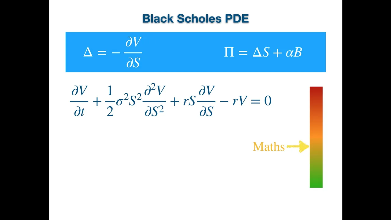
Black-Scholes PDE Derivation via Delta Hedging
@quantpie
41.3K views•2019-06-16

6:00
The Mathematical Impossibility of Accurate World Maps
@Vox
23.3M views•2016-12-02
Related Study Plans & Knowledge Roadmaps
Structured learning paths in Mathematics
mathematics
Tensor Calculus: Vectors to Riemann Curvature
01Mathematical Foundations: Linear Algebra & Calculus
02Covectors, Dual Spaces, and Tensor Basics
03The Metric Tensor and Index Gymnastics
+ 2 more learning modules
40h5 modules
Explore Roadmap
mathematics
Gödel's Incompleteness: Logic, Proofs & Limits
01Introduction to Formal Systems & Hilbert's Dream
02Set Theory, Cardinality, and Cantor's Diagonal Argument
03Arithmetization and Gödel Numbering
+ 2 more learning modules
14h5 modules
Explore Roadmap
mathematics
Galois Theory: Fields, Groups & Solvability
01Foundations of Abstract Algebra: Groups & Fields
02Polynomials & Field Extensions
03Splitting Fields & Symmetries
+ 2 more learning modules
24h5 modules
Explore Roadmap
mathematics
Non-Euclidean Geometry: Models & Geodesics
01Euclid's Fifth Postulate and the Birth of New Geometries
02Hyperbolic Space and the Poincaré Disk Model
03Geodesics: Defining Straight Lines in Curved Spaces
+ 2 more learning modules
15h5 modules
Explore Roadmap