






![[ĐGNL] VẬT LÝ | BUỔI 1 | ÔN THI ĐÁNH GIÁ NĂNG LỰC HÀ NỘI VÀ TP.HCM | HSA & V-ACT](https://i.ytimg.com/vi/CuEUxwmPID4/maxresdefault.jpg)



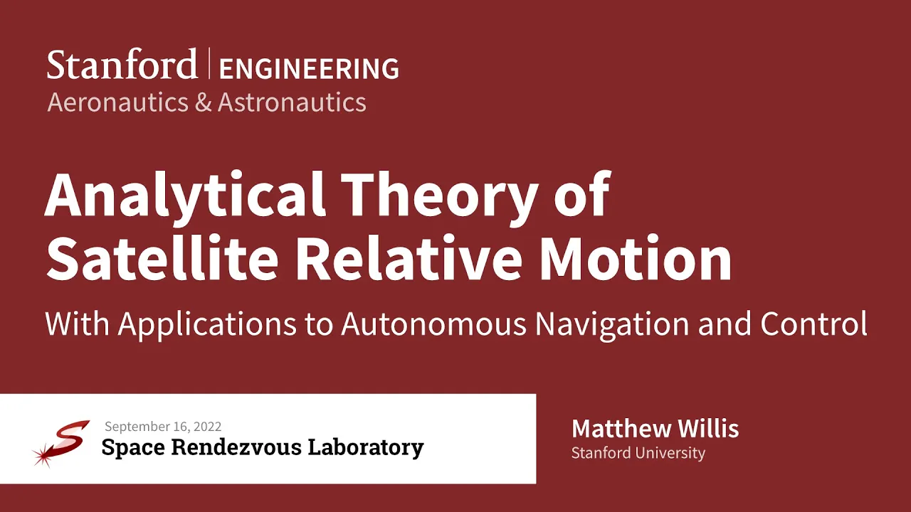







This lecture covers the fundamental coordinate systems used in satellite communications including Geographic (latitude/longitude/altitude), Cartesian, Earth-Centered Inertial (ECI), and Earth-Centered Earth-Fixed (ECEF) systems, followed by Keplerian orbit theory including the six orbital elements (semi-major axis, eccentricity, inclination, right ascension of ascending node, argument of periapsis, and true anomaly), and introduces orbital propagators such as the Keplerian two-body model and the SGP4 algorithm for simulating satellite orbits over time.
Satellite Orbits, Coordinate Systems, and Propagation | Lecture 2
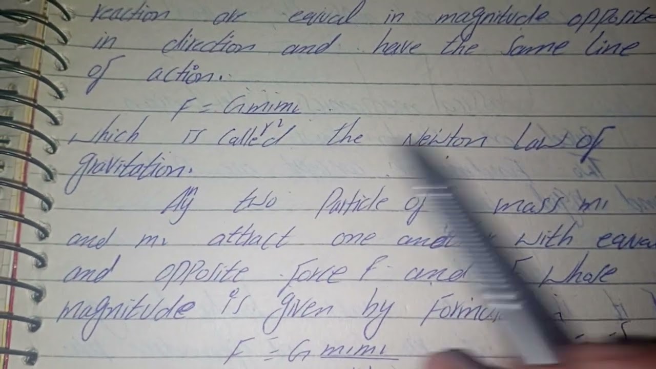
Added:Fundamentals of Newtonian mechanics, specifically Newton's laws of motion and the law of universal gravitation.
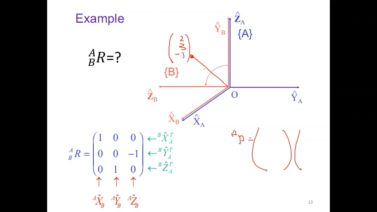
Basic linear algebra and vector calculus, focusing on 3D coordinate frames, vector operations, and rotation matrices.
Introductory MATLAB programming skills, including matrix manipulation, script writing, and basic data visualization.
Elementary physics concepts of circular motion, angular momentum, and conservation of energy.
Orbital perturbation analysis, exploring non-spherical gravity (the J2 effect), atmospheric drag, and solar radiation pressure.
Orbital maneuvers and trajectory design, including Hohmann transfers, bi-elliptic transfers, and orbital plane changes.
Orbit determination and tracking algorithms, such as Kalman filtering and least-squares estimation based on ground-station observation data.
Spacecraft attitude dynamics and control systems, studying how satellites maintain or change their orientation in orbit.
9.1K views135likes51:05Original Release: 2023-07-12
welcome to week two one important topic in Satellite Communications is the satellite orbit itself now before we understand the orbits we have to look into few of the coordinate systems that are used to describe such orbits after that we will look into the typical keplerian orbits and the elements that can describe a certain orbit its inclination its rotation its radius and so on after that we will look into propagators or if you want simulators that can simulate a satellite orbit if you give it the time and you give it the the required propagation when do you want to expect the satellite to pass after that we will look into the satellite Axis or the tracking of the satellite that is if you have a Ground Terminal what is the location of the satellite with respect to the Ground Terminal so that means if I am Ground Terminal what is the adimos and elevation of a satellite and what is the range between myself I was a Ground Terminal and the satellite these are very important parameters for later on for communication link calculations I hope you'll enjoy this lecture with me we will first start with the most common coordinate system which people some people call it the GPS coordinate system like someone asking you what is your GPS coordinates well the actual name or the correct name should be Geographic coordinated systems and the answer would be latitude longitude and your altitude so let's have a look here closer look at what are these three parameters so suppose you have you are at this point your latitude will describe your angular spacing between the Equator of Earth and your point your longitude will describe the spherical angle between a certain reference line which is called a datum or the prime meridian towards your location now that datum or prime meridian is near to Greenwich in UK and as you can see here there is a photo someone standing at exactly a longitude of zero now for these are well described in the wgs 84 system which defines the standard datum used in the geographic coordinated systems now for a satellite the SLI can still be described as well in a longitude latitude and altitude of course it will not be on the Earth's surface it will be far above Earth in our day-to-day experience it's much easier to describe points in terms of their distance in meters or kilometers and here comes the second coordinate system which we're going to talk about is the local Cartesian coordinate system so suppose you have a bunch of points here this is near to Melbourne and these points are described in terms of the latitude and longitude and someone asks okay so what is the distance between two points here it's really hard to intuitively understand that however if I used these are the same points if I convert them into a Cartesian coordinate system it's much easier to see the distance between two points here or the the average distance between the points however in order to do this conversion you need a reference point so I provided here reference point and then these all these circles are referenced towards this point and you see here the reference point has the coordinates accordance of zero zero now it's worth mentioning that the y-axis in this particular conversion is aligned with the north Direction and the x-axis is aligned with the East Direction now you can use Matlab to do this conversion so these are called conversion between lla or latitude longitude altitude to local Cartesian coordinates and you you typically you need to use a reference system such as the wgs84 system and also you need to specify a reference point where they want this Cartesian coordinates to be referenced to the previous two coordinate systems can be used for satellite or can be used for typical day-to-day activities however for satellite applications there are two coordinate systems that are much easier to use to describe a satellite orbit or a satellite location the first coordinate system is called the earth-centered inertial so in this coordinate system the satellites are independent of the earth rotation so because a sunlight they don't care if the Earth is rotating or not for them the satellites all what they care is about the mass of Earth so in that sense the ECI or air-centered inertia is fixed with respect to the Stars to the contrary the Earth's centered Earth's fixed EC EF according a system is rotating along with the Earth so that you can see here the blue one the blue coordinates are rotating with respect to the ECI frame we will see much more details in the upcoming two slides the figure on the right side shows both the ECI and the ecef coordinate systems so now as an observer we are fixed with respect to the ECI frame so here's the ACI and the ACI frame is fixed with respect to far Stars okay now let's see where this axis of the ecis are pointing let's start with the z-axis is the easiest axis so the z-axis is fixed with respect is aligned with the Earth rotational axis so that's the axis where the Earth is rotating about now the X and Y plane so X Y plane is then aligned with the equatorial plane of Earth okay now how do we point the X and Y Direction Where Do We point x why is it point to this particular location well there are different reference points where you can we can Orient your X vector one of the references for example is called the j2000 where they the x-axis is pointing to the vernal equinox at a particular time on the other hand the earth-centered Earth fixed coordinate is fixed on the earth so it is rotating along with the earth rotation so here the fixed refer to the it's fixed with the Earth and what you can see here the z-axis is also aligned with the rotational axis of Earth the x-axis passes from the point at this point here which is having a latitude of zero and longitude of zero and the X Y plane is also in the equatorial plane aligned with the equatorial plane traffic now the ecef coordinates completes one rotation every 86 164 seconds which is a if you do the math this is approximately approximately equal to 24 hours multiplied by 60 Minutes multiplied by 60 seconds now you'll find there's a difference here because actually our actual experience of a day has to do with the illumination of the Sun but the rotation of Earth itself is slightly different it's called one side real day it's slightly different than the actual our actual experience of a solar day now we will see in the lab how to do the conversions between the ecef and the ECI it's worth noting here if you have a point or a satellite that is described in the ECI frame and you want to convert the coordinates from ECI to ecef you need to know the time where do you want to do the conversion because at different time points you will get different results the last coordinate system that I would like to cover is called the adimos elevation range system this is a very important coordinate system perhaps the most intuitive way to describe the position of a satellite with respect to a ground station so we are standing at this point on the Earth's surface here is the north Direction here's the east south and west now the elevation of the satellite if you look at the sky the the this the angle between the Horizon so this circle represents the Horizon between the Horizon and the satellite is called the elevation angle now the rotation of the satellite with respect to the north so the north is the reference point when you rotate clockwise with respect to the north this is called the adimos and then the range is the distance between you as an observer and the satellite these Corners are quite important for satellite communication and as we will see also in the lab we can convert between all the previous coordinate systems in using built-in functions or also you can build your own functions to do this conversion one way to show the positions of satellite with respect to a crown user is a sky plot what is a sky plot in the sky plot you are sitting at the center of this plot and let's say if we have a satellite at this particular point it shows here that our atomos is 30 degree you see here this point 30 degree and our elevation is 20 degree so the distance or the angular distance between the Horizon so this circle represents the horizon and as you go away from the Horizon so we have zero we have 20 degree 40 degree we have 60 degree and then finally here we have 90 degree so this point represents the Zenith means if you have a satellite at this point it means it is right above your head let's take another example this point is or this satellite is at an atomos of 120 degree and an elevation at of 40 degrees you can do this exercise you can go ahead and do this exercise using Skype plot command in Matlab there is also there are also software or apps you can download in Android for example this is a nice app called gnss status it will show you the position the current position of different gnss satellites jnss mean such satellite.gps grown as or Galileo or Baidu it will show you their positions with respect to you your phone in a particular moment for example let's take this satellite this look like it's a GPS satellite GPS brn5 at this particular moment it was at an atomos of 30 degrees and an elevation so I assume this would be the Horizon this will be 30 degree elevation 60 degree elevation and 90 degree so that's that light for coincidence is around atimos of 30 and elevation of 30. on the other hand let's look at this satellite this is at adimos of 120 degrees and elevation of 60 degrees it's not a surprise that Earth is not a perfect sphere but rather it's a last slightly oblated because of the rotation of Earth so what you'll find that the radius between the center for example the distance between the center and the North or South pole is a bit shorter than the center and the equatorial plane for this reason when we convert between lla longitude latitude altitude to local Cartesian or to ecef or other coordinate system we need to take into account the obliveness of the earth and that is the Earth is not an ideal sphere we will use the wgs-84 as the reference ellipisoid so this shape is called an ellipisoid it's a slightly pressed sphere from the North and South bottoms which touched on the types of orbits in the previous lecture let's do a quick refresh and dive in more depth on these types of orbits so we have first the geostation in orbit which rotates with the earth rotation so it completes a one rotation approximately every 24 hours so it appears almost stationary for an observer on Earth we have them medium earth orbit and we gave example of GPS and Galileo constellation and finally we have the low earth orbit which are used typically for communication satellites and also for Earth observation orbit is a simple method to describe the rotation of a Celestial body in our case the satellite they are reference to Johannes Kepler and can be derived based on Newton's classical law of gravitational force which you have it from high school the force acting between two masses M1 and M2 is proportional to the masses and inversely proportional to the square of the distance between the two masses equiplier in orbit takes the form of an ellipse in this ellipse we have Earth at one of the centers of the ellipse note that the ellipse has two centers and the satellite taking rotating around Earth in an elliptical orbit the point where the satellite is the closest to Earth we call it the perigee the point at which the satellite is furthest to Earth we call it the apogee not also that a an ellipse has two semi semi-axis so one axis called the semi major axis which is denoted as a is the distance between the center and the apogee are descended with the furthest point in the ellipse and the distance between the center and the closest point of the ellipse we call it the semi-minor axis and is usually denoted as B now what happens here if a equal to B we will end up with a circle and the two Focus points of the ellipse collapses to the center so there is a parameter called the eccentricity which describe how elliptical an ellipse is what does that mean if you substitute a equal to B in this relation what you will get is eccentricity of zero eccentricity of zero refers to a circular orbit you will get a perfect circle last Concept in this slide is the true anomaly the true anomaly is the distance the angular distance between the satellite position and the perigee line one of the interesting observation of Kepler is that celestial bodies travel or sweeps equal areas in equal interval what does that mean in our context for satellites let's assume you have a satellite at this point and let's call it A1 and let's assume after five minutes we check the location of the satellite we found it at this position B2 so the area is Switched by the satellite listen denote this area as a and let's wait some time and then again check the position of the satellite and let's say the satellite is at a position A2 as I'm pointing to and after five minutes we check the position of the satellite we found it at a position called let's call it B2 now the area is swept by the satellite between A1 and and sorry A2 and B2 you will find that this area is exactly equal to the first area a third example if a satellite at the third time interval is at position A3 and after five minutes it says a position B3 what you will find that the area Swift in this five minutes is equal to the second and the first areas so this can also be deduced using Newton gravitational rules this is called the Kepler second law another concept I would like to introduce that we will use later is called the equivalent principal Circle if the principle circle is a circle orbit so if I replaced this elliptical orbit with a circular orbit with the same period This is called the principal Circle a third important observation of Kepler is about the period of the orbit how much time does the celestial body require to complete a full rotation around the the other Celestial body so in our case we have Earth and we have this the satellite so the question here or the law is about the time required for the satellite to return back to the point it started with so what the law say that the period is 2 pi square root of the semi major axis so a is the semi major axis of the ellipse so here's the same major axis this is a and um and you use the parameter called the MU mu is related it's a gravitational or standard gravitational parameter and is related to the planet that the satellite is rotating around for example for earth is known to be 3.9 Etc and for Mars there is another parameter so for each planet you will find there is different mu and that depends of course on the mass of that planet this is a nice application of the Kepler's Third Law it's asking us to calculate the altitude of a geostationary orbit and it's providing us with the length of a set real day in hours minutes and seconds and also providing us with the equatorial radius let's make a simple sketch showing the different parameters so remember it's your stationary orbit if you place the satellite in a geostation in orbit it will rotate first of all it's a circular orbit and it will rotate at the same rate as the Earth's rotation so here's another point which is called the satellite subpoint so what I'm taking here this is a slice of Earth add the Equator so this is the equatorial Circle now this asking us to calculate H which is the altitude of the Geo satellite I'm going to put here in Geo that's this x is the center of Earth that's the satellite subpoint so m equals just SS and it's giving you also the radius or the average radius of Earth at this equatorial plane which is about 6378. now it's also giving you the side real day which is the amount of time required for Earth to rotate around itself and you'll find okay why this is not 24 hours because we explained previously that our experience of the solar day is different than the rotation of Earth because solar day depends also on the rotation of Earth around the Sun now let's see what can we do for that first of all we obtain the period so if you take 23s hours multiplied by 60 Minutes multiplied by 60 seconds Plus 56 minutes multiplied by 60 seconds Plus four seconds so if you do this calculation you will end up with something similar this is provided with fraction which is a bit more accurate all right now we have the period this is the amount of time that the satellite should be rotating around Earth can we use the capital third low to calculate now the radius of that orbit well if you remember the law says if you have an orbit with a semi-major axis of a what you do you Cube that you divide it by the gravitational constant of the planet you take the square root you multiply by 2 pi and you end up with the period t but now we have t we want to obtain a easy no problem so we just rearrange this equation and you end up with this equation this one shows the relation between the semi major axis now remember this is a circular orbit so basically this is the radius of the orbit based on the period of the orbit so this if you do the calculation we'll end up with this amount now this is the radius this is not the altitude the question is about the altitude I'm just gonna I'm gonna draw the same drawing here but from Top View so what you'll see here this is this is not to scale all right so here's the orbit here's the satellite and here's the satellite subpoint now we calculated the total distance what we want is the height which and we have the earth radius so we calculate the overall distance which we called it the semi major axis so all what you need to know to do now is to subtract re from the A and that's what the third step is doing is taking the total radius subtracting re so then you can obtain the altitude of the satellite this is a very important number and you will see that we are going to use it in the upcoming lectures also in the labs an elliptical capillarian orbit can be described using six parameters and naturally we call these parameters are keplerian elements now we're already familiar with some of these elements we saw how the semi measure axis describe the ellipse we saw also how the eccentricity describes the ellipticality of an ellipse when we saw that if we have an eccentricity of zero the ellipse collapses into a circle while if you have an eccentricity of one the ellipse becomes a parabola it's not really useful for satellite communication but just to let you know that the eccentricity has a value between 0 and 1.
now the third parameter is called the inclination which describe how the orbit is rotated or inclined with respect to the equatorial plane so in this figure we're showing the satellite orbit this is the orbit of the SATA in blue and as this plane is the orbital plane and then also showing in green the equatorial plane and remember the equatorial plane is the plane passing through the equator and also is aligned with the X Y axis of the ECI frame and the AC EF frames now the angle between these two planes is called the inclination the fourth parameters is called the right Ascension of the ascending node all right it's a mouthful of a term but let's say let's see what is the ascending node what's a node so the node is the point where the two equal two planes intersects the plane of the satellite orbit and the equatorial plane we have two nodes one is called the ascending node and not here this is the direction of the satellite so the the point where the satellite goes from the south hemisphere to the north hemisphere we call the ascending and the node the point where it's going from the north hemph here to the South here to the southern hemisphere we call it the descending node now we don't really care about this so the angle that is formed between the ascending node and the reference x-axis of the ACI frame is called the right Ascension of the ascending node why is it right because going to the right direction this is the and it's usually denoted as Omega so note that this is rotation along the z-axis of course the fifth parameter is the position of the periapsis now what is the periapsis well periapsis is just a perigee remember the perigee is the closest point between the satellite and the earth center now this is not 90 degree maybe in this drawing it shows it as it is very close to 90 degree this could be anywhere so if you rotate the orbit in the direction of my movement of the pointer this is called the periapsis now these five parameters are sufficient to describe the orbit itself but then we need to have a sixth parameter which describe the position of the satellite within the orbit and this is the initial true anomaly which if you remember I'll show you the anomaly is the angular distance between the periapsis of the perigee and the satellite now we have six elements these six elements can describe the position of the satellite perfectly within an orbit this is an interactive example of player in orbit so we can see here the Earth we can see the x-axis the y-axis and the satellite position here is in a small red point this is the z-axis of Earth this is the rotational axis of Earth now the orbit is said to be as exactly as the radius of Earth so first parameters is this new measure axis I'm going to increase that so you see here the semi measure axis is increasing and now because we have a circum perfectly circular orbit so the semi measure axis is equal to the radius of the orbit okay let's have non-circular orbit we can have that by increasing eccentricity so when I increase the accent Etc this is not what's happening the orbit is becoming more like an ellipse now remember in an ellipse the Earth's center here occupies one of the focus points and in this case this Focus points of the ellipse now let's continue with the parameters so here we can see the satellite more clear if I increase the inclination look what happened so that's the inclination of the orbit is changing now how about the argument of periapsis so the argument periapses if you look at the previous slide change the rotation of the orbit within the orbit itself so look at that so I'm changing now the small Omega so it's changing here is the orbit is rotating but the angle the rotational axis is perpendicular to the to this orange plane which is this plane of the orbit now if I increase the big Omega which is the right Ascension of the ascending node the orbit will rotate around the blue or the the the z-axis which is perpendicular to the blue um to the equatorial plane which is the blue plane look what will happen now I'm increasing that so you see the the orbit is rotating around the Z axis for small Omega the orbit is rotating around the axis of the orbit itself now let's have a look at the um let's set this so some nice value for example 90 degrees and let's have a look at the satellite when we change the true enormous so this is the initial true anomaly so here I'm increasing the anomaly the position of the satellite is changing the orbit is not changing but the initial position is changing so here we have the true anomaly is zero and if I rotate it this is 180 degree let's put it 180 degree so it should be on the opposite side and if I rotate it all the way back it will come back to the perigee point you can also create an orbit using Matlab as an example so what I'm providing here for you a custom made function called gen orbit which I wrote previously that accepts different elements so this is the six elements let's have a look at this code in details so basically I'm just defining the Earth's radius and the height or the altitude of the orbit and if you add the average Earth ratios plus the height you end up with the semi measure axis so that's our first parameter I'm also entering the eccentricity I'm having an inclination the Omega this is the small Omega which is the argument of periapsis and we have the big Omega which is the right Ascension of the ascending node and also we have the initial true anomaly so in total we have six parameters describing the orbital the orbit of the satellite and then also I'm putting the MU of Earth which is the standard gravitational parameter of Earth number of periods that I would like to simulate for example here I want one period and the provocation time step so I need to simulate every 10 seconds of that orbit and also I want to simulate the orbit one full orbital period so that's why I'm calculating the orbital period based on the provided a and mu so also we have a parameter called T which is the time series now if you feed the parameters and elements to that function it will produce for you and orbit and you can plot this orbit so it's a homework for you to try this example that I have attached with this course so you can download this from canvas in this slide I'm showing a comparison between the online tool that we saw in couple of previous slides versus the Matlab code that I've provided you and you can see when you import these parameters you get same results now in real life satellite applications we use what is called the two line elements now why they are called two line elements because they are two lines and this is kind of a de facto standard of EX of describing satellite orbits you can go for example to this website and you can download freely for free all the current satellites that are orbiting Earth but they all will be in the two line element format now if you look at the two line element format it includes the six Kepler and other elements but also includes other parameters that will help you to calculate the orbit in more accuracy using different methods than the keplerian method so what we've learned so far is how to find an orbit base on Kepler motion however we will see that because Earth is not perfect sphere it has also a regular gravitational field so some areas are having more gravity than other areas we're also having some atmospheric drag that is because some the atmosphere does not stop at a particular altitude it's gradually Decay into space so satellites are pressured a little bit with the atmosphere especially low earth orbit satellites also there is a radiation pressure from the Sun and also there's a gravitational field from the Sun and the Moon so when this is taken into account you need more advanced and it's very hard to do manual calculations for this so we use codes to simulate the satellite orbits so in order to simulate the satellite orbit you need to feed it with the two line element this is an example of the International Space Station it's Internet space station and code word zarya you can download the updated two light elements from this website this is an example on how to use the two line elements and feed them to Matlab such as it can produce for you in orbit now this is a built-in function in Matlab so what do you need to feed it with the start time and for example this is a start time that I selected for the simulation the stop time when the simulation you want to end and I will simulate here for two hours the sample time how much the interval between the sampling point so the lesson number they will take more time to simulate because you have more samples the higher the number the the accuracy will be lower but it's okay for our illustration purpose and then you need to create the scenario now this example is just a rough example in during the lab you will go into much details how you originate your own orbits and you will study it in much more detail originating the satellite scenario and then we are generating the satellite and after that we are displaying that satellite so if you run this video you'll find this is the International Space Station based on the downloaded elements from the website that I've mentioned before an orbital propagator is a tool it's a simulation tool that you need to feed it with the elements of the orbit that describes the orbit for example in the previous example we fed with the capillary elements we also fed it with the time of simulation so and then it produced for us and orbits a satellite orbit now similarly we saw another example where we fed a tool with the tle two line elements and also we provided the start and the end time of the simulation and also we found the orbit and that was a simulation for the ISS station now in the upcoming a couple of slides we will dive in deeper on how these two different orbital propagated now these are simple this is a very simple provocative the capillarium propagator we will also look at another propagator called the scp-4 but there are also other many other propagation methods that are out of the scope of this course the first propagator that we'll look at is the two body propagator which is the simplest propagator and also called the keplerian propagator it assumes that Earth has a uniform gravitational field it means the Earth mass is uniformly distributed and actually you can collapse the whole math at the center of Earth and what does that mean this is based on Kepler's observation that the orbit will be in a perfect ellipse shape there are two steps to generate the orbit first you need to generate an ellipse because we know that the orbit is an ellipse but second you need to rotate that ellipse there are three rotations that you need to apply for the ellipse so the first rotation you need to rotate so here's the base here's the ellipse now the first rotation is that ellipse need to be rotated so from this state it will become as here's the Earth again it will be rotated and this rotation we called it the argument of periapsis rotation the second rotation we need to rotate the orbital plane itself against the equatorial plane so I'm going to draw an occupatory plane and here is the orbital plane and this angle between them we call it the inclination now the third orbit so this is the first the second is the inclination the third rotation that we need to do is we need to rotate the orbit itself around the z-axis and we call this rotation as the right Ascension of the ascending node now you don't have to do this don't worry about them this is for your info the upcoming slide this is for info of how to generate an orbit yourself how to design a propagator yourself however in all the examples that will be provided you will use a built-in propagator in Matlab this is for you to understand in more depth how the orbits work let's have a deeper look into how to generate a keplerian orbit this first step as we said is to generate the base orbit which is an ellipse in order to draw an ellipse you need to know the semi-major axis which is an input parameter and also the eccentricity e a satellite at the beginning as we said it's at an angle Nu which is the true anomaly and at a certain distance let's call it r so what we need to do now is to find the series of points on this ellipse that the satellite would be positioned at at every time instance so for example if you have a time Vector let's call it from 0 and 1 second two seconds three seconds Etc and up to the last end point would be T So at Point T the satellite will return back T is the orbital period the cell will return back to the starting point so what we need to know we need to know the radius r at each of these time intervals and we need to know the new angle or the true anomaly at each of these time intervals so if we can build these two vectors so Vector means a series of data if you can build these two vectors then we can draw the orbits there are a couple of steps needed before we can generate our Vector R vector and new Vector remember these vectors are needed such that we can generate an ellipse first let's remember the concept of the principal Circle we introduced that a couple of slides ago so what is the principle Circle it's a virtual orbit that if you placed a satellite at the virtual orbit and here's your real cell line approach in blue both the blue satellite will have a orbit T and the virtual satellite will have orbit orbit period t but the nice thing about this virtual orbit that it has a uniform circular motion so what does that mean if you want to know the mean anonymity we call this the mean anomaly with the position of the virtual satellite if you want to know this mean anomaly all what you need to know then is the time T so in one period capital T the satellite will make 1 4 Circle so Omega 2 pi so in a small time T the satellite will simply make t over capital T multiplied by 2 pi so what does that mean it means they mean anomaly of the virtual satellite is simply 2 pi small T divided by capital t plus the initial mean anomaly and according to Kepler so I'll show you the difference between the true anomaly and the mean anomaly so remember a Kepler said if for equal a period you will pass equal areas so at this point I'm going to draw this in blue this is your actual satellite after let's say two time clicks it's a disposition now the red satellite after two time clicks it is at this position so if you run the simulation the virtual satellite will pass this amount in angles and the actual satellite will pass this amount so I'm just going to draw it on top of it in terms of angles so so the true anomaly at this point is equivalent to the mean anomaly at this point at a certain time simulation time equal to D there are three equations here in this slide that I'm not going to provide the proof for them you can refer to any of the orbital mechanic books and you'll if you are interested in the detail proof but what these three equations tell you that if you have the expression for the mean anomaly or if you have the vector of the mean anomaly and yes we do because remember we have the T Vector which is that simulation time for example we're simulating 0 5 Seconds 10 seconds Etc up to a period T you can calculate the M Vector from it and we saw the simple equation how to calculate it was just 2 pi T over capital t plus the initial mean anomaly so we know M so this equation will tell you you can calculate what is called The Eccentric anomaly which is denoted here as e and based on The Eccentric anomaly you can calculate the true anomaly and the radius of the orbit remember these are what we needed for generating an ellipse now these are polar coordinates so let me just review what we said if we have a simulation time Vector T for example 0 5 10 seconds Etc up to a period T you can then deduce the vector R which is the distance between the earth center and the satellite and also you can deduce the vector Nu which is the angle between the x-axis and the satellite so if you are making here a simple drawing I want to convert these polar coordinates into Cartesian coordinates so all what you need to do here is the r here is angle Nu here's the satellite let's call it here set and this point at the center is Earth so the and here's the x-axis here's the y-axis so basically X is simply R multiplied by cosine U and the Y value is R multiplied by sine U now the orbital plane this is the Base plane where you're generating is still in the X Y plane so the orbital plane is still in the X Y plane so that's why all the z's are zero we will see in the upcoming slides how we will rotate the space orbit in three dimensions we will see here an example of how the three rotations are applied as part of step two so first look at the white orbit this is the base orbit and you can see the base orbit now is aligned with the X Y plane the first rotation is around the z-axis here's the z-axis and we're going to rotate with an amount small Omega which is the argument of the periapsis so note here the rotation is happening around the z-axis here's the z-axis and we rotate it with an amount small Omega the second rotation is around the x-axis and will be with an amount of the inclination and see what will happen so this is the x-axis the green line and now I'm rotating and see what's happening I'm rotating around the Green Line the third and the last rotation is around the Z again so here's the Z axis and I'm going to rotate within a month big Omega which is the right Ascension of the ascending node and see what will happen it's rotating around the z-axis now of course in the simulator here it doesn't matter which order of rotation you apply however when you're writing the script the rotation should be in order so you end up with the correct orbits the second propagator that we are going to use in this course is called the scp-4 algorithm which stands for the simplified General perturbation algorithm now explaining the details how this algorithm work is beyond the scope of this course but if you are interested there are papers explaining how the algorithm works now this algorithm is much more accurate than the keplerian motion or the two body motion because it takes many aspects into consideration for example it takes the gravity and you're non-uniform gravitational field of Earth now this is not a new algorithm it was developed in 1970s and it was secret but then it was it was made public in 1980s and there were also new improvements even at recent 2020 the nice thing it is is relatively fast and computer computationally efficient but it is not faster of course than the keplerian algorithm so keplerian algorithm is very simple and it's much faster to obtain to calculate than the sgp4 now there are more advanced propagation algorithms which also require more simulation time or more calculation time now given its popularity you can find codes in both Matlab and python to generate the sgp4 so all what you need to do is to input as we saw at the beginning input the tle elements also input the start and the end so the simulation time to the sgp4 and then you can get the position of the satellite at different time instances we will see an example in the next slide how to use Matlab built-in function in Matlab to generate an orbit let's walk through an example in Matlab of how to generate an orbit and propagate that orbit using scp-4 and using the two body keplerian method so first I'm starting by clearing the variables and closing the windows so I'm just putting the word hidden here because the if any previous window opened by the satellite simulator will be closed now we need to specify when you want to start a simulation when do you want to stop it so I'm putting in some arbitrary date here so you can put the year month day and hours minute seconds the stop time is the start time and I added I won't simulate the orbit for 30 minutes you can of course increase and decrease now this is the sampling time so I'm asking the simulator to simulate every second between in this 30 minutes now this command will create the scenario which with the start time the stop time and the sampling time which is one second now what I'm going to do I'm going to create two satellites the first satellite so I defined an altitude of around 400 kilometers so I added on top of the earth radius the I identified the eccentricity to be zero so that's a circular orbit now I defined inclination the right extension of the ascending node the argument of pre-apses and toronomy Etc so now I'm creating the satellite and so I I fed all these parameters so you can of course check the documentation you always can press on the function and press F1 or can you can Google it so you can see the syntax of how to write the commands now if you scroll here I didn't specify anything else so let's try I'm gonna start one by one so now I'm just clearing I'm creating the scenario now created a satellite so let's have a look here what do you see here we see the satellite parameters and then we see the orbital propagator so by default Matlab uses sgp4 now let's play the scenario so this will take a minute to load now when it loads so is it loading and so let's rotate here here is the satellite as we just created so you can change the time playing speed and you can advance the time and see where the satellite would be now note here the orbit seam looks like earthy looks like fixed but it's not really the case look at the background so the stars are moving so our camera is fixed on Earth um so that's why we're seeing the Earth is not rotating but actually you can change also the setting so you can fix the background and makes the Earth rotating so that's the homework for you to try now let's continue I'm going to create another satellite but this time at the end I'm gonna specify that I need a two body keplerian propagator so you see here orbital orbit propagators and um I specifying the two body capillary so let's run this um and at first I'm gonna close the um so that's maybe optional so let's try to run it without closing yep so you don't need to close it so let's look at the second satellite I created it so it specify the fabric address too by the capillarium now let's go back to the um I know we put in two set both satellites so the first satellite is using the HTTP 4 the second is using the keplerian now note there is a slight difference between the two orbits this is due to the different implementation in Matlab for these two propagators um now on the long run now this might be some programming thing in in implementing the orbits but on the long run these orbits will deviate each other so if I run this for for example 20 or 30 for example rotation or orbits you'll find that two satellites will have different location of course the as we saw in the lecture the two body propagator is less accurate than the sgp4 algorithm a typical satellite antenna can rotate in the elevation and the azimose direction so what we've done in the previous slide we have shown different methods to calculate the satellite orbit now we will see how we will use the satellite orbit to point the antenna towards the satellite in a low earth orbit satellite the satellite is passing for a short period let's say within 15 minutes The Horizon of the user so this is a typical satellite dish or satellite antenna and you can see the mount here there is an elevation motor so here's the elevation motor that can rotate the antenna up and down so it will change the elevation angle but also as you can see from this mod this mod can rotate around the atomos so here this Mount can rotate around the SMS so if you input certain adimos and elevation to the controller the controller will point the antenna towards the satellite and remember in the Leo satellite you have to keep active tracking for the satellite if you want to communicate with that satellite during a given period and also we say that geost satellites and we will see that in the um in the simulation that Geo satellites are also moving slightly and thus require also some kind of tracking especially if you have a very large antenna with very narrow beam width I have modified a bit the previous satellite scenario so now we have a better orbit passing near to Melbourne so you can play the scenario and you can see the satellite is moving so what I'm going to do now is I'm going to create a ground station so this ground station is I took the coordinates of rmit University so if I add this not here so we'll now have a ground station here in the CBD so what I'm going to do now is to track the satellite with respect to this particular ground station so in particular I would like to know the edimos and elevation of that satellite with respect to the ground station so you can also obtain the range which is the distance this is very important later for calculating the free space path laws for communication for calculating the signal attenuation between satellite between the satellite and the ground station what I'm doing also here I'm creating a Time Vector so basically this is just a a Time variable so if I run this with F9 so what you'll find here is that just the time will be nicely presented as the x-axis so I'm plotting here the elevation across the time so here's the time it's 8 minutes and here's the satellite path so in during the simulation time the elevation of the satellite started from around 6 went all the way to around 20 and then back to zero so note that you could have a negative elevation that's okay but that means the satellite is not visible it's below the horizon now we can also upload the satellite pass in the polar coordinates so in the polar coordinate remember that this point is the Dennis is the point above our head directly above our head so it is 90 degrees 0 is the Horizon so that Circle here is the Horizon and that Arc here is the arc where the satellite start and ends its pass we have reached the end of this lecture thank you for watching looking forward to see you in the upcoming lectures
Up Next
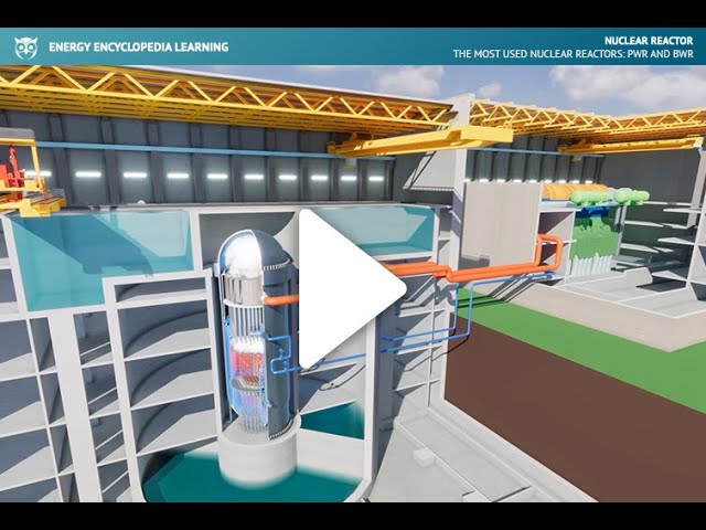
7:38
PWR vs. BWR: Pressurized & Boiling Water Reactors Explained
@energyencyclopedia
83.5K views•2023-10-18

30:32
Ultrasonic Transducers: Resonant Frequency Measurement and Horn Design
@imajeenyus42
229.9K views•2017-02-22

54:16
Polymer Environmental Degradation: Mechanisms & Stabilization
@iit
1.8K views•2012-07-10

33:39
How a Student's Question Saved a NYC Skyscraper from Collapse
@veritasium
22.8M views•2025-04-26
Related Study Plans & Knowledge Roadmaps
Structured learning paths in Engineering
engineering
Building Acoustic Levitators: Physics & Arduino
01The Physics of Sound and Standing Waves
02Piezoelectric Transducers and H-Bridge Drivers
03Arduino Programming: Generating 40 kHz Signals
+ 2 more learning modules
14h5 modules
Explore Roadmap
engineering
Building Peltier Cloud Chambers: Particle Tracks
01Cosmic Rays & Cloud Chamber Physics
02Thermoelectric Cooling (TEC) Fundamentals
03Custom Liquid-Cooling Loop Design
+ 2 more learning modules
18h5 modules
Explore Roadmap
engineering
Yagi-Uda Antennas: Modeling, Build & VNA Test
01Introduction to RF and Antenna Fundamentals
02Yagi-Uda Antenna Design Principles
03Antenna Modeling and Simulation in 4NEC2
+ 2 more learning modules
18h5 modules
Explore Roadmap
engineering
ECG Monitor Design: Op-Amps, Filters & Noise
01Electronics & Breadboard Basics
02Op-Amps and Instrumentation Amplifiers
03Bioelectricity and ECG Fundamentals
+ 2 more learning modules
18h5 modules
Explore Roadmap