PID (Proportional-Integral-Derivative) control is essential for self-balancing robots, where the three parameters Kp (proportional gain), Ki (integral gain), and Kd (derivative gain) work together to maintain balance: Kp responds to current error, Ki eliminates steady-state error over time, and Kd predicts future errors based on rate of change; proper tuning involves adjusting these values iteratively to achieve stable, responsive balancing without oscillation or delay.
PID Tuning for Self-Balancing Robots: A Practical Guide
Added:Deep Dive
Fundamentals of feedback control loops, specifically how an error signal is used to adjust system inputs.

00.00 Course introduction and syllabus
4.8K
Feedback control systems measure the actual output, compare it to the desired output (command), and use the error signal to adjust the input. The error is calculated as the difference between the commanded value and the actual output. The controller processes this error and determines the appropriate input to the system to reduce the error. This closed-loop approach provides robustness against modeling errors and disturbances.
Click to watch →

Traditional Advanced Control - Part 6
1.5K
A feedback control loop consists of an output measurement affected by both input and disturbance. The system uses the difference between the setpoint and actual output as an error signal, which the controller acts upon to generate an input to the process. When error is zero, no control action is needed. This closed-loop approach enables both disturbance rejection (maintaining output value when disturbances occur) and servo control (following setpoint changes).
Click to watch →

Arduino PID Controller - From Scratch!
104.5K
The error signal is the fundamental input to any PID controller. It represents the difference between the desired setpoint (target value) and the actual measured value from the process. The controller's entire purpose is to reduce this error to zero or within an acceptable tolerance. For example, if the setpoint is 75 and the actual reading is 60, the error is +15, indicating the system needs to increase its output to reach the target.
Click to watch →

Instrumentation and Control Technician Training - Fundamentals - Basic Control Loops
1.6K
With feedback control, when the controlled variable changes away from set point, an error signal is generated causing the controlling element to produce a signal that adjusts a manipulated variable and returns the controlled variable to set point. The feedback feature becomes evident after the error has been detected, and the control loop acts to correct the error. If the controlled variable continues to move away from set point or begins to return to set point, the primary element also senses these changes, then the measuring element produces a signal proportional to this change, feeding back this signal to the controlling element which compares it with set point and adjusts the final control element to correct the error based on the new signal.
Click to watch →
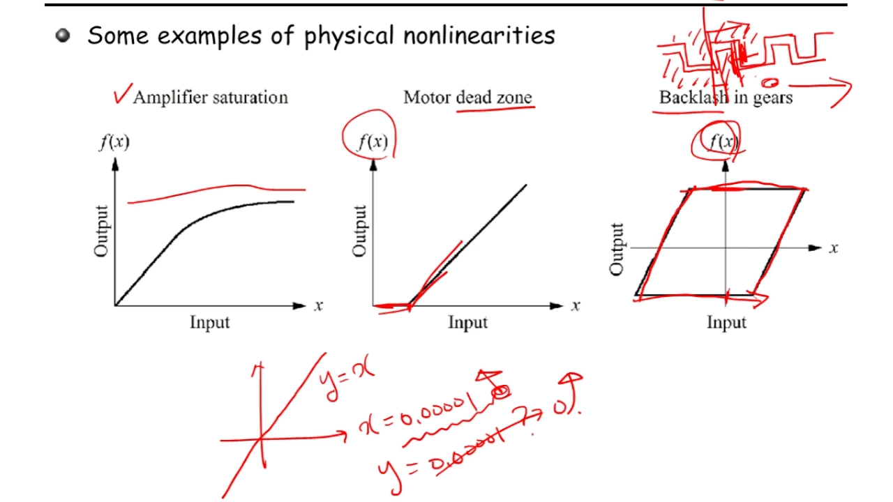
EMSE301 자동제어 ch2_9 (Sec.2.10~2.11: Nonlinearities and Linearization, 비선형성 및 선형화)
3.2K
The error signal is the difference between the desired value (setpoint) and the actual measured value in a feedback control system. The error signal is calculated by subtracting the measured value from the desired value. This error signal is then fed into the controller, which processes it to generate the appropriate control action. The controller's goal is to minimize the error signal by adjusting the system's inputs.
Click to watch →
Deep Dive
Basic mathematical understanding of Proportional (Kp), Integral (Ki), and Derivative (Kd) control actions.

PID Controller Explained: Basics, Block Diagram, Transfer Function
176K
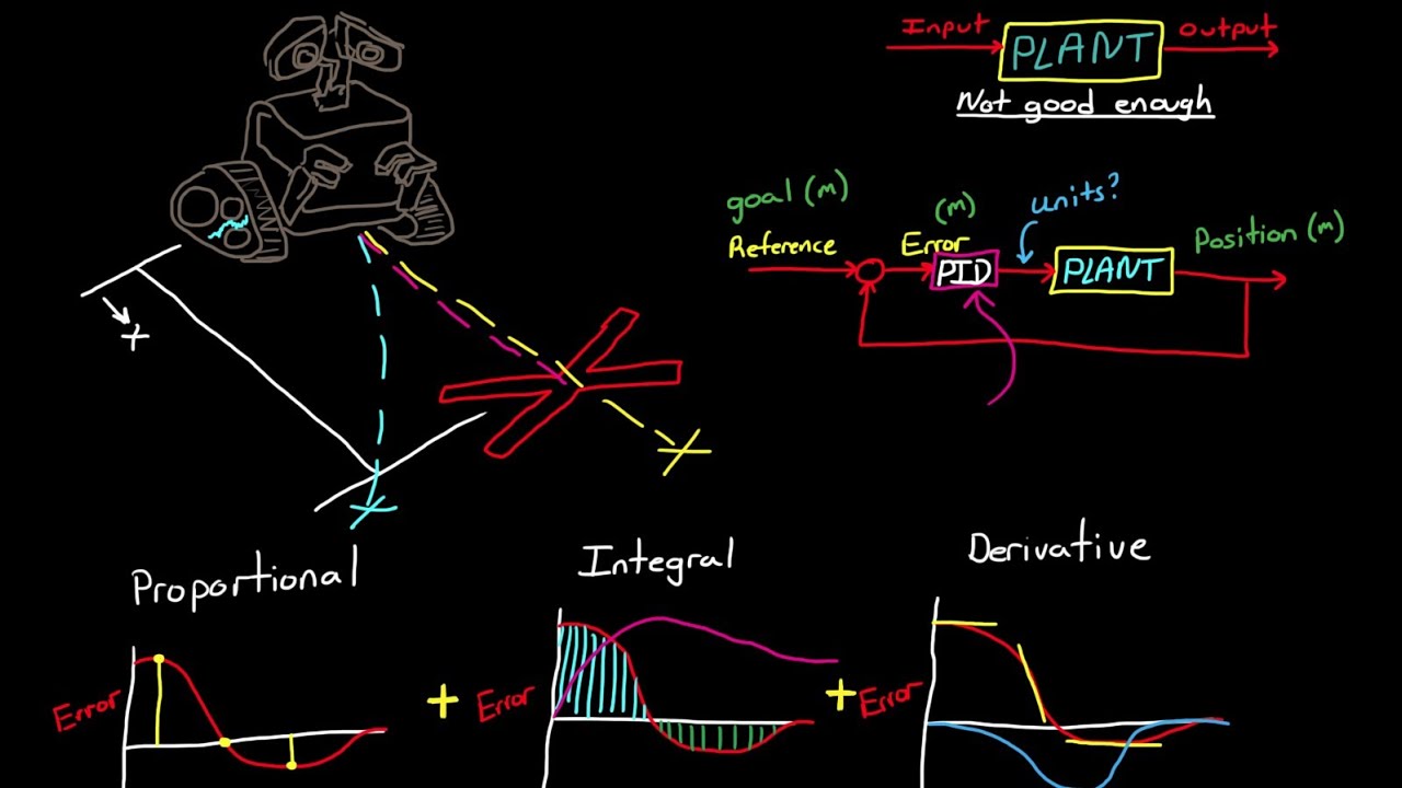
This section explains the physical mechanisms behind each P controller component. The proportional action (KP×error) provides immediate response proportional to current error, with output shape depending only on error magnitude. The integral action (KI×∫error dt) accumulates positive and negative areas over time, increasing output during positive error periods and decreasing during negative periods, which eliminates steady-state error. The derivative action (KD×d(error)/dt) responds to the slope of the error signal—producing zero output at constant error, decreasing during negative slopes, and increasing during positive slopes—enabling predictive control that anticipates future errors based on their rate of change.
Click to watch →
PID Control - A brief introduction
1.7M
The proportional action produces an output directly proportional to the current error magnitude—large errors produce large corrective outputs. The integral action accumulates past errors over time and multiplies them by Ki, effectively eliminating constant steady-state errors since even small persistent errors accumulate to significant values. The derivative action responds to the rate of change of error, producing larger outputs when errors are changing rapidly, which helps anticipate future error trends and improve stability.
Click to watch →

전기기사 제어공학 1강 1~12P | 제어계의 기본 구성, 자동제어계의 분류, 1장 문제풀이
130.1K
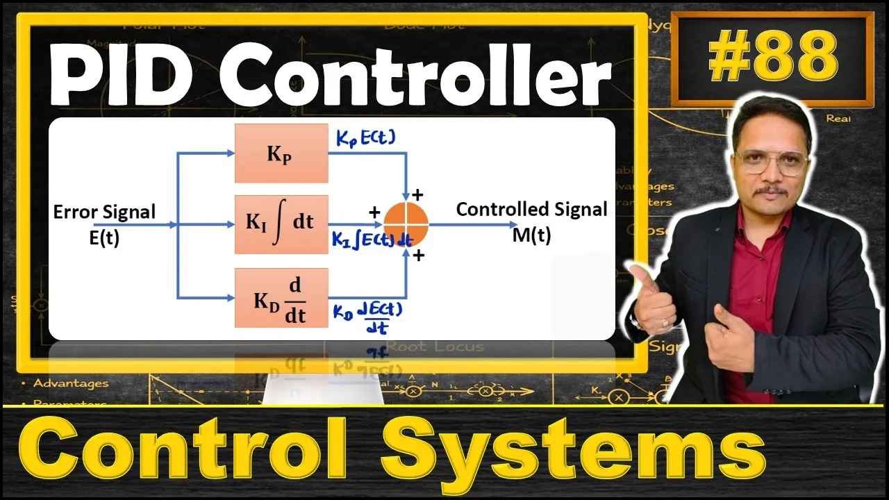
Three fundamental control actions form the basis of PID controllers: (1) Proportional control (P) - the output is proportional to the current error value (output = Kp × error), providing immediate response but leaving steady-state error; (2) Integral control (I) - the output is proportional to the integral of the error over time (output = Ki × ∫error dt), eliminating steady-state error but potentially causing overshoot and slow response; (3) Derivative control (D) - the output is proportional to the rate of change of the error (output = Kd × d(error)/dt), anticipating future error trends and improving stability. Combining these actions creates PID control, which balances rapid response, steady-state accuracy, and system stability.
Click to watch →
PID Controller Explained: Basics, Block Diagram, Significance, Transfer Function, Pros, and Cons
13.9K
Proportional action scales the input error by a constant KP without changing its waveform shape. Integral action accumulates past error values over time, causing continuous increase when input is positive, decrease when negative, with rate dependent on input magnitude. Derivative action measures the slope of the error signal, producing output proportional to how fast the error is changing—positive slope gives positive output, negative slope gives negative output, and zero slope gives zero output. These three mechanisms work together to provide comprehensive error correction.
Click to watch →
Proportional (P), Integral (I) and Derivative (D) control actions
758
PID controllers use three fundamental control actions—Proportional (P), Integral (I), and Derivative (D)—to regulate system dynamics: P control responds to current error with output proportional to error magnitude, I control eliminates steady-state offset by integrating past error over time, and D control anticipates future error by responding to the rate of change of error, with each action affecting system response characteristics differently (P affects rise time and overshoot, I eliminates steady-state error, D improves stability but amplifies noise).
Click to watch →
Deep Dive
The physics of an inverted pendulum system, including gravity, torque, and rotational inertia.

Unstable inverted pendulum: modelling, linearization, free response (Laplace)
238
This segment covers the complete physical modeling process for an inverted pendulum system. The system consists of a rigid body with moment of inertia J and mass M, articulated at a fixed pivot point. The gravitational force mg acts at the center of gravity, located at distance L from the pivot, creating a torque equal to mgLsin(α) where α is the angular displacement. Newton's second law for rotational motion states that J times angular acceleration equals the net torque. The video explains how to write the fundamental differential equation governing the system's motion, including both gravitational torque and any manipulated torque from a motor. This establishes the mathematical foundation for all subsequent analysis.
Click to watch →

2.2 Ejemplos de linealización: Sistema escalar y péndulo invertido
1.9K
The inverted pendulum consists of a mass attached to a fixed pivot point by a rigid rod. The system is described by variables including the vertical position, angular position (θ), external torque applied to return the pendulum to vertical position, mass (m), rod length (l), gravitational acceleration (g), and moment of inertia (J). The dynamic model is derived using Newton's laws and contains a nonlinear term (sin(θ)), making it a nonlinear differential equation.
Click to watch →

SISTEMAS DE CONTROL - Estabilización Mecánica del Péndulo Invertido
4.4K
When inverted, the weight force creates a destabilizing moment, yielding θ'' - (g/L)θ = 0 with hyperbolic solutions showing complete instability. Adding viscous friction (moment proportional to angular velocity Bθ') and a perturbing force, the complete differential equation becomes mL²θ'' + Bθ' - mgLθ = F(t)L. Block diagram representation shows positive feedback from the tipping moment, which inherently destabilizes the system. The transfer function θ(s)/F(s) = L/(mL²s² + Bs - mgL) reveals that friction alone cannot stabilize the position due to the strong overturning moment.
Click to watch →

12. Classical Mechanics | CSIR NET & GATE Physics Lectures
534
The equation of motion for the inverted pendulum is ml²θ_double_dot + mlAω² cos(ωt) cosθ - mgl sinθ = 0. This is obtained by applying the Euler-Lagrange equation to the Lagrangian. The term mlAω² cos(ωt) cosθ comes from the coupling between the pendulum motion and the support motion. The term -mgl sinθ is the gravitational torque.
Click to watch →

A Self Balancing Robot Story
1.1K
In an inverted pendulum system, gravity always acts downward. When the bar rotates even slightly, there is a distance between the center of the pivot and the center of mass of the bar. Since gravitational force acts at some distance from the pivot, it creates a torque that causes the pendulum to fall down. This demonstrates why an inverted pendulum is inherently unstable and requires active control to maintain balance.
Click to watch →
Deep Dive
Familiarity with sensor-actuator hardware, particularly reading angle data from an IMU (gyroscope/accelerometer) and driving DC motors via PWM.
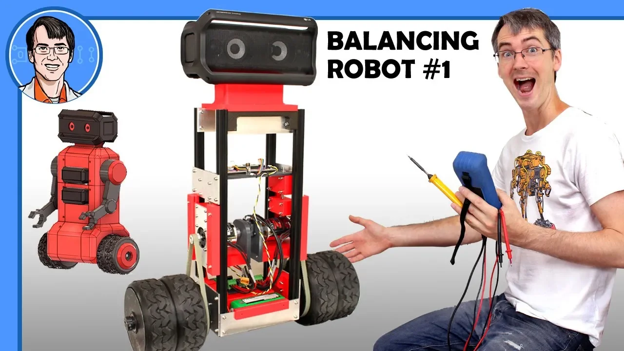
Building a Two-Wheel Balancing Robot | with LG XBOOM Go Speakers
100.8K
The MPU 6050 inertial measurement unit provides accelerometer and gyroscope data combined into angle measurements. Using interrupt service routines allows efficient data acquisition where the IMU signals when data is ready, enabling the main loop to read angles only when necessary rather than polling continuously.
Click to watch →
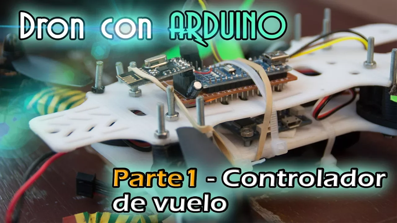
Pr#006 Dron con Arduino - Parte 1 - El controlador de vuelo
201.3K
This tutorial demonstrates how to construct a drone flight controller using an Arduino Nano microcontroller and MPU6050 inertial measurement unit. The system reads sensor data from the MPU6050 (gyroscope and accelerometer) to calculate the drone's orientation, then uses PID control algorithms to adjust four brushless motors via electronic speed controllers (ESCs). The MultiWii open-source firmware provides the control logic, while the hardware setup includes connecting the MPU6050 via I2C (pins A4/A5), ESC outputs on digital pins 3,9,10,11, and a PPM signal input for the radio receiver. The final configuration involves calibrating the accelerometer and setting PWM signal ranges (1000-2000 microseconds) for motor control.
Click to watch →
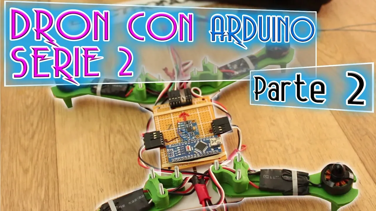
Pr#36 Dron Arduino - Serie 2 | Parte 2 IMU y PID
21.6K
This comprehensive section covers the complete process of reading and processing IMU data from the MPU6050 module. The process begins with establishing I2C communication by importing the Wire library, configuring the slave address (0x68), and resetting the device by writing to register 0x6B. The tutorial explains how to read gyroscope data from registers 0x43-0x46, combining high and low bytes to form 16-bit values, then dividing by 32.8 to convert to degrees per second. For accelerometer data from registers 0x3B-0x3F, the same byte combination technique applies, with conversion by 4.096 to obtain g-forces. The section addresses critical calibration by zeroing gyroscope offset through averaging 200 readings, and demonstrates integrating gyroscope velocity values to obtain actual angles. The Euler angle formula is introduced for calculating inclination from accelerometer data, and the complementary filter is explained for sensor fusion between gyroscope and accelerometer readings.
Click to watch →
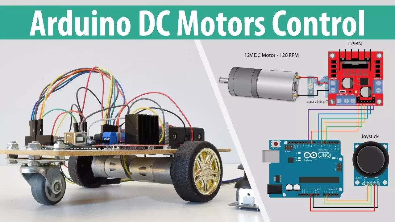
Arduino DC Motor Control Tutorial - L298N | H-Bridge | PWM | Robot Car
1.3M
This tutorial explains how to control DC motors using Arduino by combining PWM (Pulse Width Modulation) for speed control and H-bridge circuits for direction reversal, with the L298N driver module serving as a dual H-bridge motor controller that accepts PWM signals on enable pins and direction signals on input pins to simultaneously control two DC motors' speed and rotation direction.
Click to watch →
Controlando a rotação de motores DC com Arduino - Curso de Arduino #19
21.9K
This tutorial demonstrates how to control DC motor speed using Arduino by mapping potentiometer input values (0-255) to PWM output values (0-255), where the potentiometer connected to analog input A0 provides variable resistance that adjusts motor speed proportionally through the PWM pin 3 connected to a TIP120 motor driver.
Click to watch →
Prerequisite Knowledge
- Concept 01Fundamentals of feedback control loops, specifically how an error signal is used to adjust system inputs.
- Concept 02Basic mathematical understanding of Proportional (Kp), Integral (Ki), and Derivative (Kd) control actions.
- Concept 03The physics of an inverted pendulum system, including gravity, torque, and rotational inertia.
- Concept 04Familiarity with sensor-actuator hardware, particularly reading angle data from an IMU (gyroscope/accelerometer) and driving DC motors via PWM.
Subsequent Learning
- Step 01Implementing sensor fusion algorithms, such as Complementary or Kalman filters, to obtain clean, low-noise tilt angle measurements.
- Step 02Mathematical system identification to model the robot's physical transfer function and analytically calculate optimal PID gains.
- Step 03Exploring advanced control theories like LQR (Linear Quadratic Regulator) and State-Space control for multi-variable stability.
- Step 04Integrating trajectory planning and navigation stack (e.g., ROS) to enable autonomous movement and obstacle avoidance while balancing.
Initial Focus
Core Concept
Key Term Reiterated
Transition Point
Engagement Call
Reinforcement
Reemphasis
Key Summary
Closing Greeting
Final Theme
Initial Focus
0:38Playing Section
- 1
Main topic is introduced with key term.
- 2
Core concept repeated for emphasis.
Model-Based Control (LQR and MPC) vs. Classical PID Control
While PID controllers are popular for their simplicity and intuitive tuning, they are linear controllers applied to a highly non-linear, unstable, and coupled system (the inverted pendulum). PID struggles with multi-variable control—such as simultaneously stabilizing the robot's tilt angle and controlling its position—and lacks robust stability guarantees. An alternative, modern control perspective advocates for model-based strategies like the Linear Quadratic Regulator (LQR) or Model Predictive Control (MPC). These state-space methods leverage a mathematical model of the robot's physical dynamics to calculate optimal control signals. LQR naturally handles multiple-input, multiple-output (MIMO) systems by optimizing a cost function that balances stabilization performance against control effort. MPC goes further by predicting future states and accounting for physical constraints, such as motor voltage limits. Shifting from empirical PID tuning to systematic model-based design allows engineers to achieve superior stability, faster recovery from disturbances, and precise path-tracking that PID struggles to deliver.
Deep Dive
Implementing sensor fusion algorithms, such as Complementary or Kalman filters, to obtain clean, low-noise tilt angle measurements.

Raspberry Pi Pico W LESSON 51: Ultimate Pitch and Roll Gadget Using the MPU6050
4.3K
A complementary filter combines accelerometer and gyroscope data to create fast, accurate, and low-noise tilt measurements by using the accelerometer as a long-term anchor (0.5% trust) and the gyroscope for short-term data (99.5% trust), while integrated error compensation removes long-term steady state drift to achieve reliable roll and pitch measurements suitable for real-world applications.
Click to watch →

myComplementary Filter
5K
A complementary filter is a sensor fusion algorithm that combines accelerometer and gyroscope data to measure tilt more accurately by leveraging the strengths of each sensor—using the accelerometer's stable long-term readings to correct for gyroscope drift while using the gyroscope's responsive short-term measurements to track rapid movements.
Click to watch →
Kalman Filter for 6DOF IMU Implementation (2/6)
11.3K
A complementary filter is a sensor fusion technique that combines gyroscope and accelerometer measurements to estimate orientation angles, where the gyroscope provides high-frequency angular rate data (with drift) and the accelerometer provides low-frequency absolute angle data (with noise), with the filter blending these signals using weighted gains (typically 99% gyro and 1% accelerometer) to produce a stable angle estimate that corrects for gyroscope drift while minimizing accelerometer noise effects.
Click to watch →
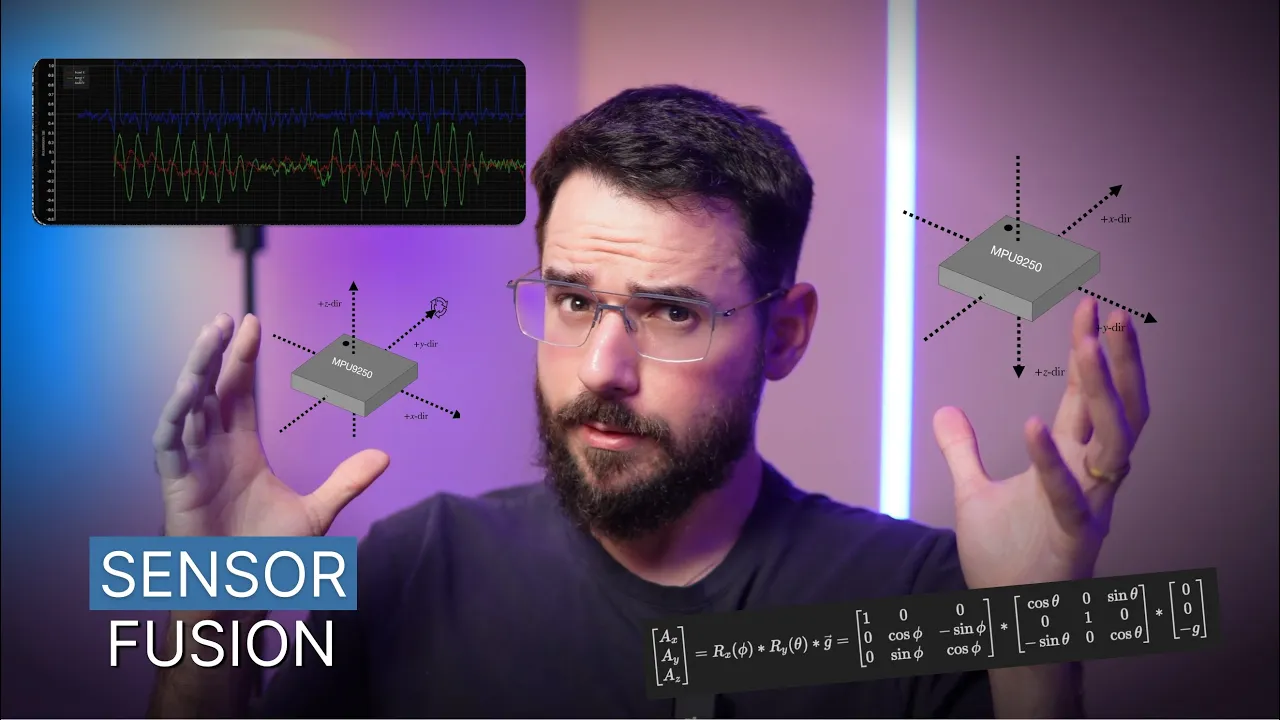
Practical Sensor Fusion
514
Complementary filtering combines gyroscope (smooth but biased) and accelerometer (noisy but correct) measurements. The filter uses a single parameter alpha to balance sensor weighting. The equation: fused_angle = alpha × (previous_fused_angle + gyro × delta_t) + (1 - alpha) × accelerometer_angle. Since alpha < 1, the filter converges toward accelerometer measurements, preventing bias accumulation. This simple technique provides smooth, accurate angle estimates suitable for most applications, solving approximately 90% of sensor fusion problems.
Click to watch →
9-Axis IMU LESSON 9: Accurate and Stable Tilt Using Accelerometers, Gyros and a Complimentary Filter
30.9K
A complementary filter combines accelerometer and gyroscope data by applying a high-pass filter to the gyroscope (for quick response) and a low-pass filter to the accelerometer (for long-term stability), resulting in tilt estimation that is both responsive and immune to vibration and drift.
Click to watch →
Deep Dive
Mathematical system identification to model the robot's physical transfer function and analytically calculate optimal PID gains.
Peter Ponders PID - System Identification Advanced
1K
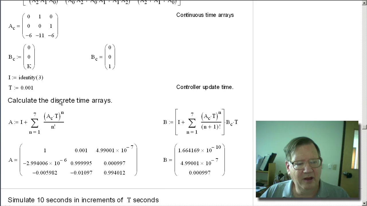
System identification is the critical first step in control system design, where engineers determine the mathematical model (transfer function) of a physical system by exciting it with known inputs and analyzing the output responses; this process involves accounting for real-world imperfections like quantization errors from digital sensors and measurement noise, then using optimization algorithms such as Levenberg-Marquardt to estimate parameters like gain and pole locations, which enables accurate controller design through techniques like pole placement and PID tuning.
Click to watch →
Robotics 1 U3 (Motion Control) S5 (PID) P3 (Analytical Control Tuning)
4.4K
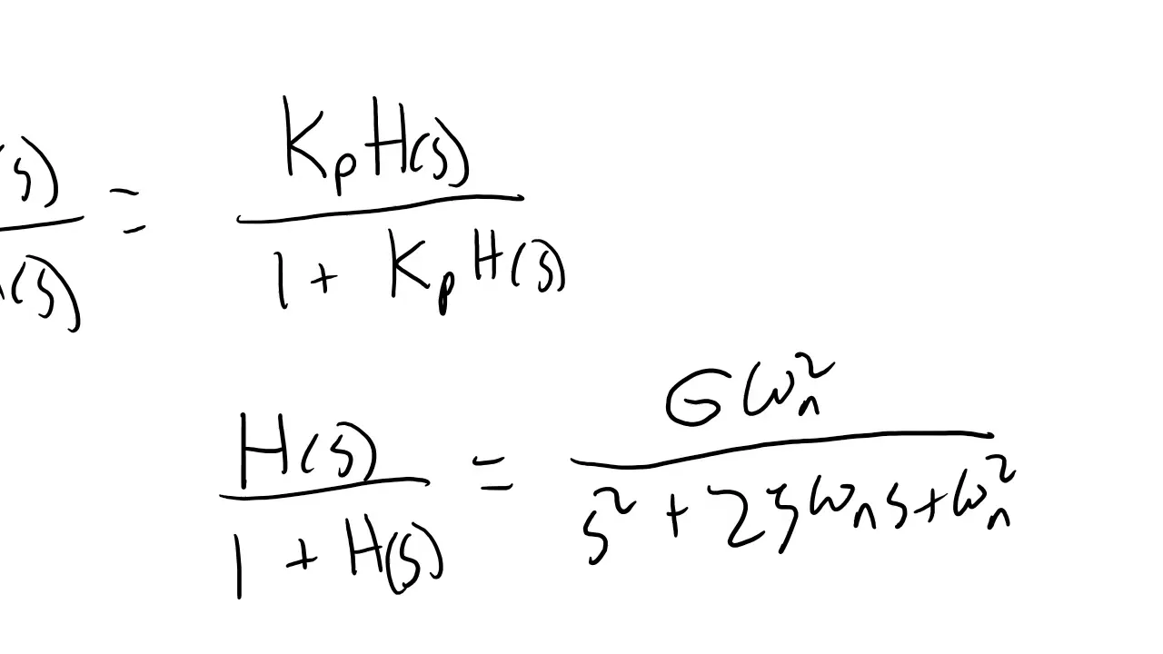
This video demonstrates how to analytically calculate the proportional gain (KP) for a critically damped response in a rack and pinion system by using step response data to create a system model, then applying Laplace transforms and block diagram reduction to derive the plant transfer function, and finally solving for KP by setting the damping ratio (zeta) to 1. The method involves finding the relationship between system parameters (gain, natural frequency, damping ratio) from the step response, then back-calculating the KP value that will achieve the desired damping. However, analytical methods rely on assumptions of linearity and infinite control loop speed, which may cause discrepancies between calculated and experimental values, requiring fine-tuning in practice.
Click to watch →

Robotic Car - A Simple Way to Build a Model
57.7K
System identification allows engineers to develop mathematical models of unknown systems through empirical testing rather than deriving equations from physics. The process involves defining clear input-output relationships (such as PWM commands to angular velocity), recognizing that true physical quantities cannot be directly measured (only sensed values are available), and using transfer functions to represent the complete system behavior. This approach enables application of linear control theory techniques for stability analysis and controller design without requiring detailed knowledge of internal mechanical components.
Click to watch →
Peter Ponders PID - System Identification Basics
2.2K
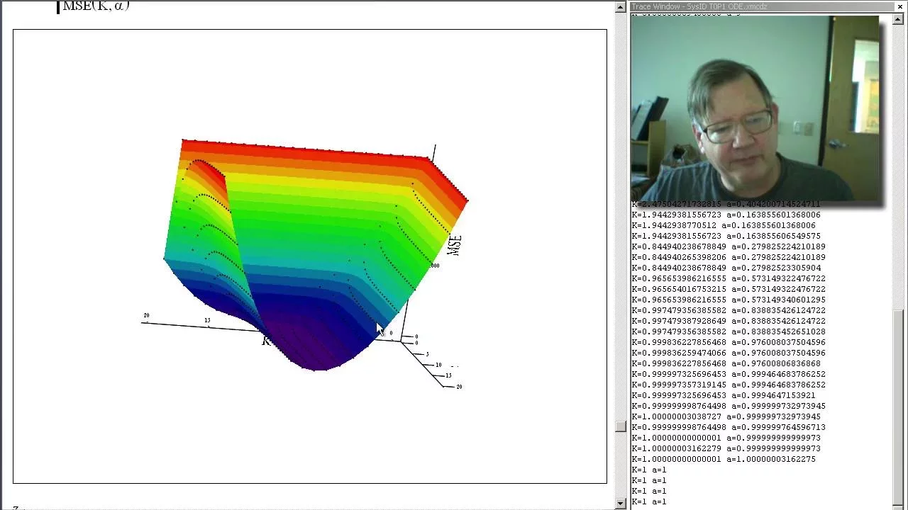
System identification is the process of determining a system's open-loop transfer function by minimizing the mean squared error between simulated and actual responses; this involves testing different model structures (integrating/non-integrating, single/multiple pole) and using optimization algorithms like Levenberg-Marquardt to automatically find optimal parameters, as manually adjusting multiple parameters simultaneously becomes impractical when working with higher-dimensional parameter spaces.
Click to watch →
The Full Modeling and simulation of a Robotic Arm using MATLAB simscape multibody and Solidworks
164.8K
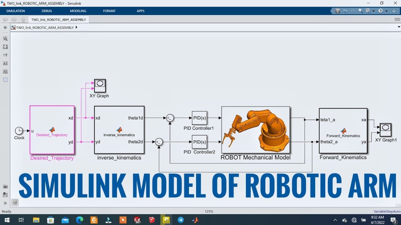
This section explains automated PID tuning using MATLAB's PID Tuner application. The process involves: (1) Pressing the tune button on the PID controller block; (2) Linearizing the nonlinear mechanical model to approximate it as a linear system; (3) Opening the PID Tuner interface showing plant response and tuned response; (4) Adjusting sliders to modify response time characteristics; (5) Observing overshoot, settling time, and rise time metrics; (6) Updating the PID block parameters with optimized values; (7) Repeating the process for multiple PID controllers; (8) Accepting suboptimal results if optimal tuning is not achievable. The tuner provides a systematic approach to finding reasonable PID parameters without manual trial-and-error, though it may not produce optimal results for highly nonlinear systems.
Click to watch →
Deep Dive
Exploring advanced control theories like LQR (Linear Quadratic Regulator) and State-Space control for multi-variable stability.

Control Theory Bootcamp 2025 | Webinar 4 - Advanced Control | Recording
167
The Linear Quadratic Regulator (LQR) is an optimal control algorithm that uses full state feedback (u = -Kx) to minimize a cost function balancing state errors (Q matrix) and control effort (R matrix), making it suitable for complex multivariable systems like balancing robots where PID controllers are insufficient due to their reactive nature and inability to handle coupled dynamics; unlike PID which only responds to errors, LQR plans ahead by considering the entire state vector, and its performance depends critically on tuning Q and R to balance responsiveness against control effort, with linear models only valid for small deviations from stable states.
Click to watch →
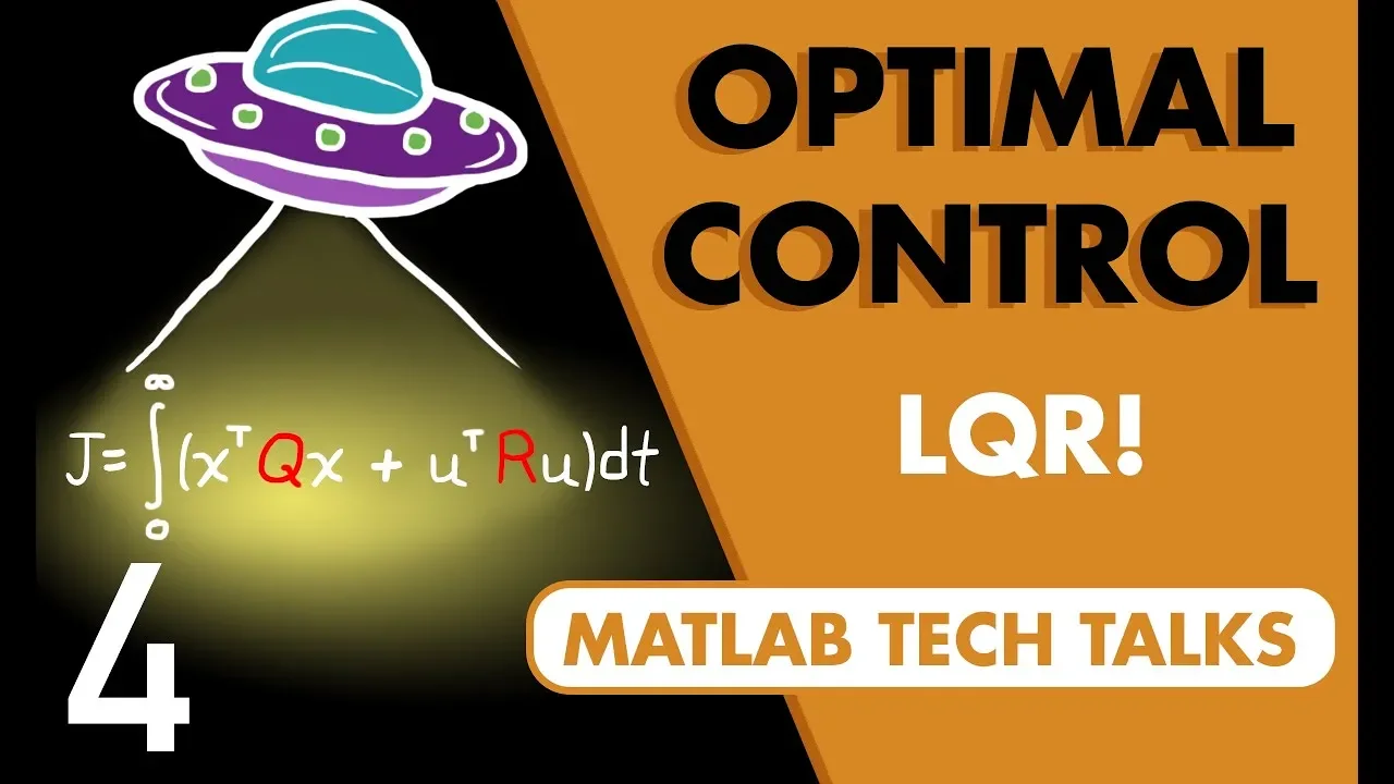
What Is Linear Quadratic Regulator (LQR) Optimal Control? | State Space, Part 4
362.1K
The Linear Quadratic Regulator (LQR) is an optimal control method that determines the optimal feedback gain matrix by minimizing a quadratic cost function that balances system performance (measured by state errors) against actuator effort (measured by control inputs), allowing designers to specify trade-offs between how quickly the system responds and how much energy or resources are consumed, rather than manually placing poles as in pole placement methods.
Click to watch →
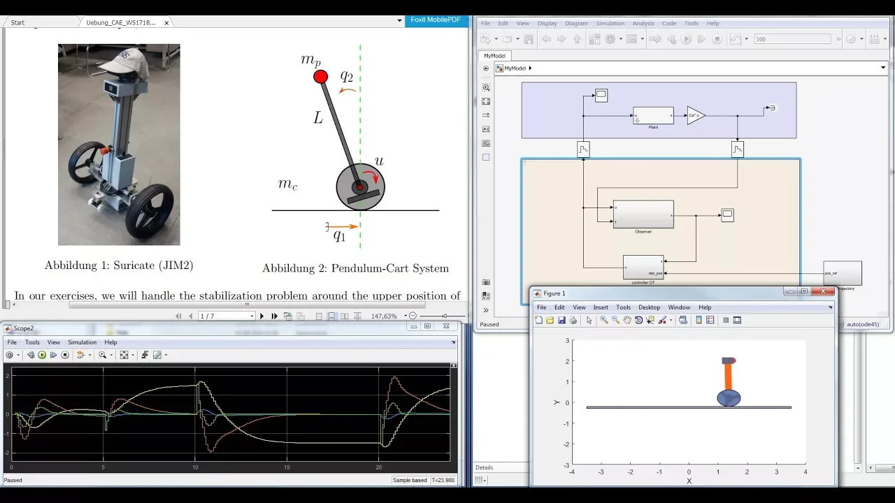
State Space Control for the Pendulum-Cart System: A short tutorial on using Matlab® and Simulink®
131.1K
LQR is an optimal control method that designs a state feedback controller by minimizing a quadratic cost function J = ∫(x^TQx + u^TRu)dt, where Q penalizes state deviations and R penalizes control effort. The controller gain K is computed using the lqr(A,B,Q,R) command. Unlike pole placement, LQR provides a systematic way to balance control performance against input effort. Increasing the weight on Q improves state regulation but increases control effort, while increasing R reduces input magnitude at the expense of slower response.
Click to watch →

GIAN Course "Modeling and Control of Power Electronic Converters for Energy System Application"
216
This section introduces optimal control via LQR: (1) LQR finds state feedback K minimizing cost J = ∫(X^T Q X + U^T R U) dt; (2) Q and R are positive definite weight matrices determining trade-off between state regulation and control effort; (3) Solution K = R^(-1)B^T P, where P solves algebraic Riccati equation; (4) LQR automatically places poles in optimal locations without manual pole placement; (5) Existence requires (A, B) controllable and (Q^(1/2), A) observable; (6) MATLAB's 'lqr' command solves this problem.
Click to watch →

Linear Systems 26: Linear Quadratic Optimal Control
1.5K
Linear Quadratic Regulator (LQR) is an optimal control methodology that designs state feedback controllers by explicitly defining a quadratic performance index to be minimized, rather than manually placing poles. The method involves solving the Riccati differential equation (for finite-horizon problems) or the algebraic Riccati equation (for infinite-horizon/stationary problems) to obtain the optimal feedback gain matrix. Key requirements include controllability/stabilizability of the system and detectability/observability for asymptotic stability guarantees. The resulting controller provides guaranteed closed-loop stability, robustness properties including approximately 60 degrees of phase margin and infinite gain margin, and allows designers to trade-off between control effort and system performance through the weighting matrices Q and R.
Click to watch →
Deep Dive
Integrating trajectory planning and navigation stack (e.g., ROS) to enable autonomous movement and obstacle avoidance while balancing.
![[ROS Q&A] 049 - How to navigate while avoiding obstacles](https://i.ytimg.com/vi/k3axKeaS66A/hqdefault.jpg)
[ROS Q&A] 049 - How to navigate while avoiding obstacles
20.9K
The ROS navigation stack enables autonomous robot navigation through a three-stage process: first, creating a map of the environment using the gmapping package by moving the robot around; second, saving the map using map_server; third, launching the navigation stack with map_server, amcl (localization), and move_base nodes together to enable the robot to navigate while avoiding obstacles by sending goals to the robot.
Click to watch →

Robot AI Demo - NVidia Deep Learning, ROS Navigation, Raspberry Pi
213K
The ROS navigation stack enables autonomous robots to plan paths from start to goal positions using costmap-based planners. Users specify goals through GUI interfaces, and the system generates planned paths displayed as trajectories on the map. The robot continuously updates its estimated position through localization algorithms and adjusts its orientation upon reaching targets. This enables complex navigation tasks including moving through doorways and around obstacles.
Click to watch →
ROS2 Nav2 Navigation Stack Crash Course for Beginners
98.5K
The ROS2 Nav2 Navigation Stack enables autonomous robot navigation through a two-step process: first generating a map of the environment using SLAM (Simultaneous Localization and Mapping) with sensor data from the robot's laser scanner, and second using this map to navigate the robot safely from point A to point B while avoiding obstacles; the stack consists of multiple interconnected components including the global planner for pathfinding, local planner for obstacle avoidance, and AMCL (Adaptive Monte Carlo Localization) for robot positioning within the map, all communicating through ROS2 topics and services.
Click to watch →
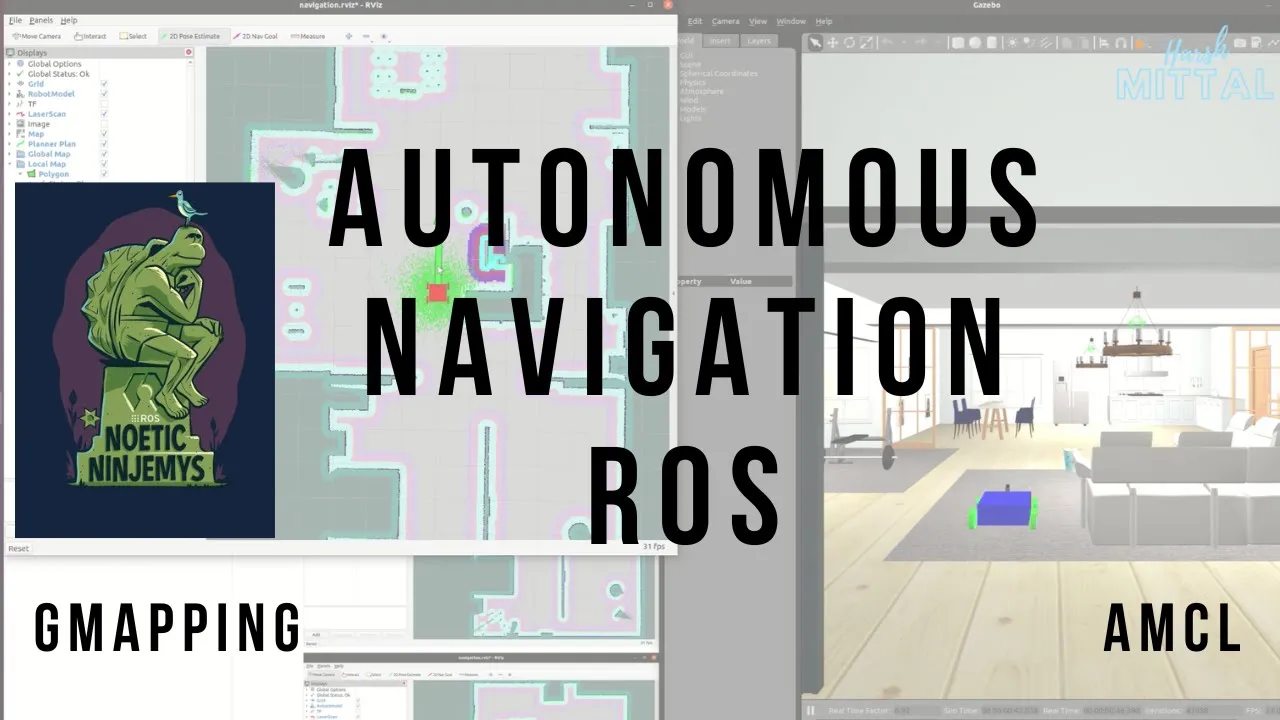
Learn Basics Of Autonomous Navigation for Custom Robot Using ROS | Simple Tutorial | 2022
10K
This comprehensive tutorial covers the complete three-stage process for implementing autonomous robot navigation using ROS. Stage 1 focuses on GMapping, a laser-based SLAM algorithm that enables robots to create maps of unknown environments while simultaneously localizing themselves. The process involves controlling the robot through teleop_twist_keyboard to capture laser scan data from multiple angles, then saving the resulting map using rosrun map_server save_map, which generates .pgm and .yaml files. Stage 2 implements AMCL (Adaptive Monte Carlo Localization), a probabilistic algorithm using particle filters that maintains a set of possible robot positions and refines estimates based on odometry and laser data, improving accuracy through movement. Stage 3 integrates autonomous navigation using the move_base node, which combines global path planning (A* algorithm) with local obstacle avoidance, using costmap parameters to represent the environment. The complete system enables robots to navigate from start to goal positions while dynamically avoiding both static and dynamic obstacles, demonstrating true autonomous operation through the integration of mapping, localization, and navigation capabilities.
Click to watch →
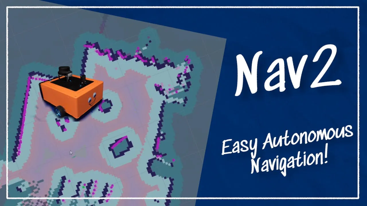
Robot Navigation Using Nav2 and ROS: A Complete Guide
173.1K
This tutorial demonstrates how to implement autonomous robot navigation using the Nav2 stack in ROS, covering the essential components: localization (via SLAM or AMCL), cost map generation for obstacle avoidance, and trajectory planning. The workflow includes setting up twist_mux for command velocity multiplexing, running navigation in Gazebo simulation, deploying on real hardware, and configuring AMCL for map-based localization. Key concepts include understanding how Nav2 uses cost maps to represent safe and dangerous areas, setting 2D goals for autonomous movement, and implementing waypoint navigation. The tutorial emphasizes practical implementation steps, including copying and customizing launch files and parameter configurations for tuning navigation behavior.
Click to watch →
Initial Focus
Core Concept
Key Term Reiterated
Transition Point
Engagement Call
Reinforcement
Reemphasis
Key Summary
Closing Greeting
Final Theme
Initial Focus
0:38- 1
Main topic is introduced with key term.
- 2
Core concept repeated for emphasis.
Model-Based Control (LQR and MPC) vs. Classical PID Control
While PID controllers are popular for their simplicity and intuitive tuning, they are linear controllers applied to a highly non-linear, unstable, and coupled system (the inverted pendulum). PID struggles with multi-variable control—such as simultaneously stabilizing the robot's tilt angle and controlling its position—and lacks robust stability guarantees. An alternative, modern control perspective advocates for model-based strategies like the Linear Quadratic Regulator (LQR) or Model Predictive Control (MPC). These state-space methods leverage a mathematical model of the robot's physical dynamics to calculate optimal control signals. LQR naturally handles multiple-input, multiple-output (MIMO) systems by optimizing a cost function that balances stabilization performance against control effort. MPC goes further by predicting future states and accounting for physical constraints, such as motor voltage limits. Shifting from empirical PID tuning to systematic model-based design allows engineers to achieve superior stability, faster recovery from disturbances, and precise path-tracking that PID struggles to deliver.
Fundamentals of feedback control loops, specifically how an error signal is used to adjust system inputs.
Basic mathematical understanding of Proportional (Kp), Integral (Ki), and Derivative (Kd) control actions.
The physics of an inverted pendulum system, including gravity, torque, and rotational inertia.
Familiarity with sensor-actuator hardware, particularly reading angle data from an IMU (gyroscope/accelerometer) and driving DC motors via PWM.
Implementing sensor fusion algorithms, such as Complementary or Kalman filters, to obtain clean, low-noise tilt angle measurements.
Mathematical system identification to model the robot's physical transfer function and analytically calculate optimal PID gains.
Exploring advanced control theories like LQR (Linear Quadratic Regulator) and State-Space control for multi-variable stability.
Integrating trajectory planning and navigation stack (e.g., ROS) to enable autonomous movement and obstacle avoidance while balancing.
354 views4likes3:01@RobusTwoMinuteTutorialsOriginal Release: 2025-12-23
Heat. Heat.
Heat. Heat. N.
Heat. Heat. N.
Come on.
Hey. Hey.
Heat. Heat. N.
Heat. Heat.
Hello.
Heat.
Up Next

17:47
FFT Sound Visualization with p5.js: Graphic Equalizer Tutorial
@TheCodingTrain
287.9K views•2016-10-19

12:54
Triumph of Orthodoxy Icon: Byzantine Art & History Explained
@BenCallan
2.1K views•2024-08-06

9:49
FastAPI vs Flask vs Django: Choosing the Right Python Web Framework
@TechWithTim
302.5K views•2024-05-26

1:42
Game of Thrones Opening Credits: A Cinematic Analysis
@gameofthrones
46.3M views•2011-04-18
Related Study Plans & Knowledge Roadmaps
Structured learning paths in General & Interdisciplinary Studies
general-studies
Elevator Engineering: History, Physics & Cities
01From Hoists to Safety Brakes: The Dawn of Vertical Lift
02Hydraulic vs. Traction: The Engineering Physics of Elevators
03Modern Speed, Safety, and Algorithms
+ 2 more learning modules
12h5 modules
Explore Roadmap
general-studies
Rubber: Material Science, History & Geopolitics
01Origins of Natural Rubber & Mesoamerican History
02The Chemistry of Natural Rubber & Vulcanization
03The Geopolitics of the Rubber Boom & Colonization
+ 2 more learning modules
12h5 modules
Explore Roadmap
general-studies
Containerization: Evolution, Logistics & Trade
01Ancient Trade & Bulk Cargo: Amphorae to Barrels
02The Industrial Revolution & Cardboard Packaging
03The Containerization Revolution: Malcom McLean
+ 2 more learning modules
12h5 modules
Explore Roadmap
general-studies
Textile Tech: Evolution, Labor & Global Impact
01Pre-Industrial Textiles: Handloom & Cottage Industry
02Mechanization: The Spinning Jenny to the Power Loom
03The Factory System & Global Labor Transformation
+ 2 more learning modules
10h5 modules
Explore Roadmap