Spectral Graph Theory: Matrices & Eigenvalues

Learning Goal: Leverage eigenvalues, adjacency matrices, and Laplacian operators to analyze complex network topologies. Uncover the structural, dynamical, and spectral properties of graphs to solve problems in network partitioning, node ranking, and graph-based machine learning.

• Prerequisites: Basic high-school algebra, introductory programming (preferably Python). No advanced prior knowledge of graph theory or machine learning is required.
• Estimated Total Study Time: 15 Hours

---

Module 1: Foundations of Linear Algebra: Vectors & Matrices

To analyze complex networks through their eigenvalues, you must first master the language of linear algebra. This module establishes a strong geometric and algebraic foundation. You will learn to see matrices not just as blocks of numbers, but as dynamic transformations that stretch, rotate, and scale vector spaces. This intuition is vital to understanding how eigenvectors characterize the foundational structures of graphs.

Recommended Videos

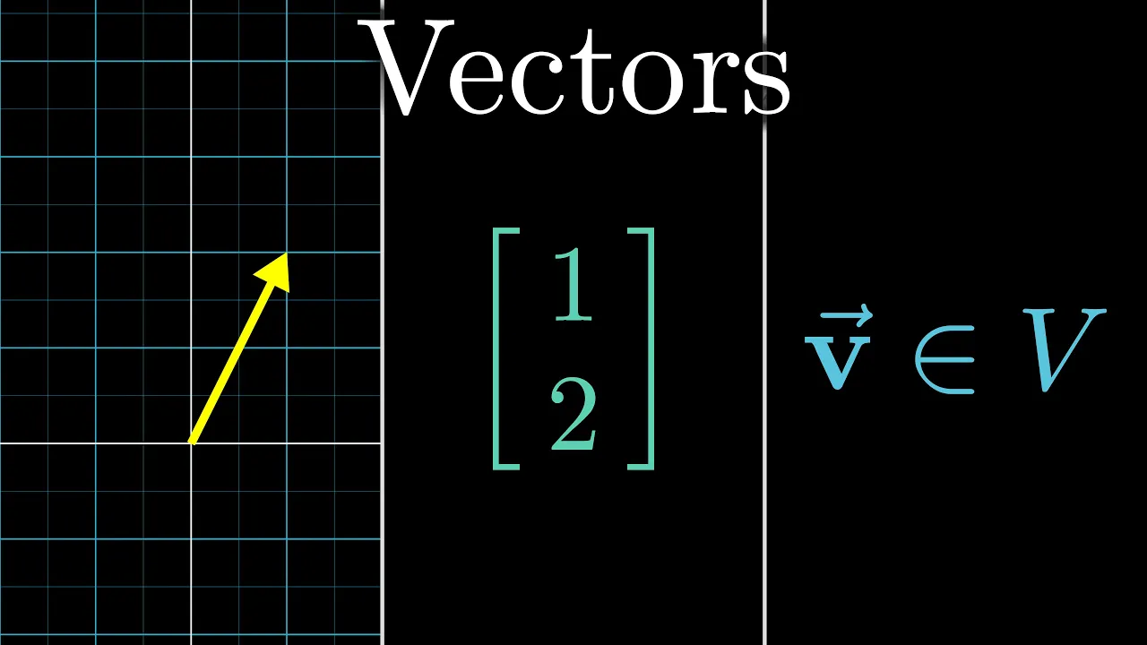
Why this video: This video provides the ultimate conceptual launchpad, illustrating vectors from three distinct perspectives: the computer scientist's list of numbers, the physicist's arrow in space, and the mathematician's synthetic bridge between the two. Developing this physical intuition of vectors is crucial before mapping them to node values on complex graphs.

Knowledge Checkpoint:

• Understand the spatial and list-based representations of a vector.
• Perform basic vector operations (addition and scalar multiplication) geometrically.
• Conceptualize how a vector can represent state values across a network.

---

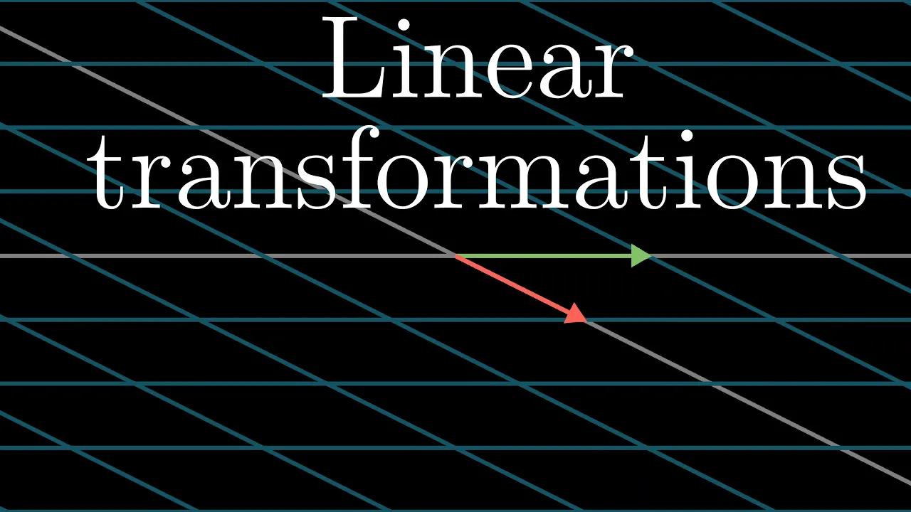
Why this video: Here, you will learn to visualize matrices as dynamic actions that transform space. Linear transformations must keep grid lines parallel and evenly spaced while keeping the origin fixed. This visual intuition is key to understanding how adjacency matrices transform structural data when they operate on graph signals.

Knowledge Checkpoint:

• Define a linear transformation and identify its geometric properties.
• Explain how matrix columns represent the destination coordinates of standard basis vectors.
• Compute the transformation of any vector given a $2 \times 2$ transformation matrix.

---

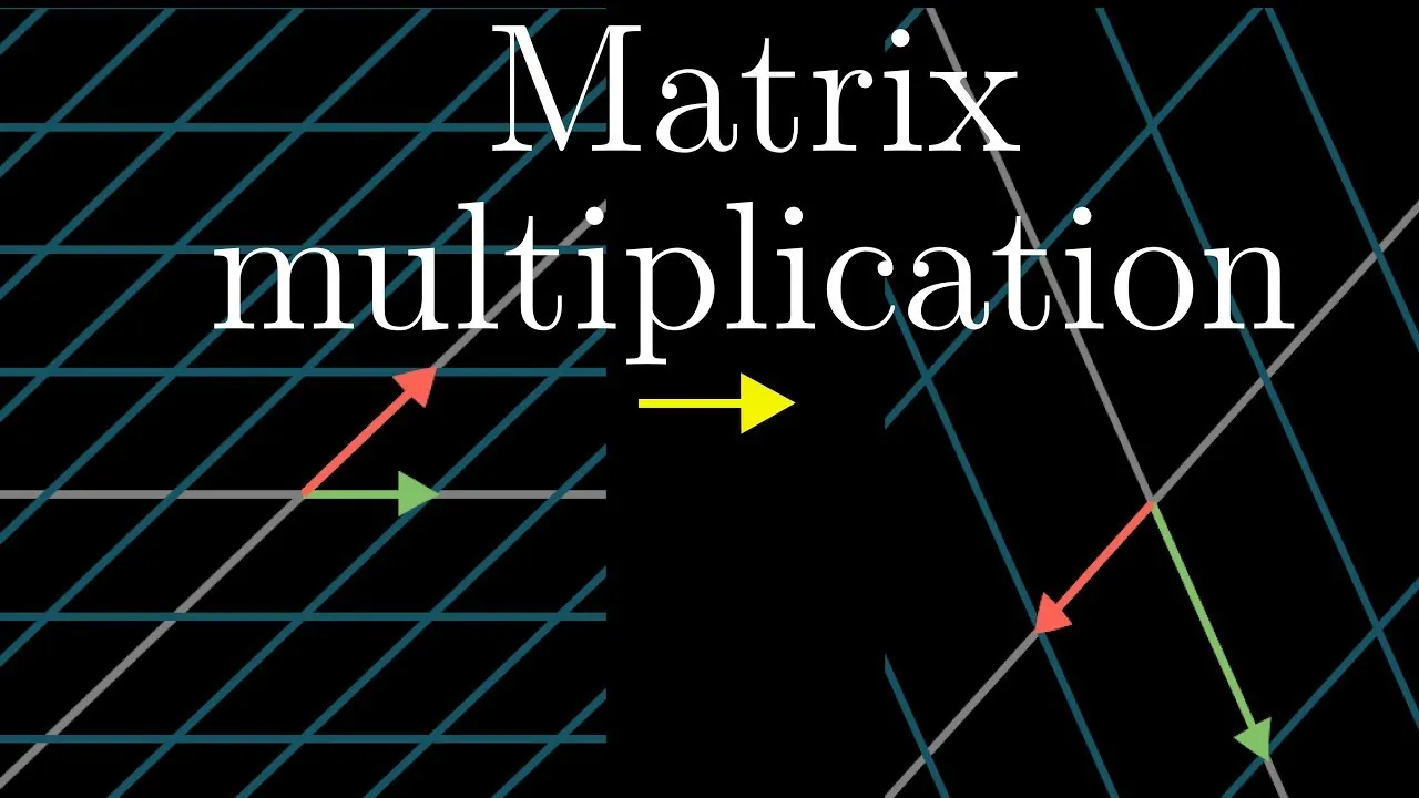
Why this video: This tutorial clarifies why matrix multiplication is structured the way it is: as the composition of successive linear transformations. This is crucial for spectral graph theory, where applying an adjacency or transition matrix multiple times corresponds to tracing multi-step random walks or diffusion processes through a network.

Knowledge Checkpoint:

• Explain why matrix multiplication is generally non-commutative ($AB \neq BA$).
• Conceptualize matrix-vector multiplication as a systemic state transformation.
• Geometrically interpret the composition of two distinct linear transformations.

---

Why this video: This video provides a clear mathematical explanation of eigenvectors—special vectors that do not change direction during a linear transformation—and their corresponding eigenvalues, which represent the scaling factor. In spectral graph theory, the eigenvectors of structural matrices act as coordinate systems that reveal a network's communities and bottlenecks.

Knowledge Checkpoint:

• Solve the characteristic equation $\det(A - \lambda I) = 0$ to find eigenvalues.
• Solve the homogeneous system $(A - \lambda I)\mathbf{v} = \mathbf{0}$ to find eigenvectors.
• Give a geometric definition of an eigenvector-eigenvalue pair.

---

Module 2: Introduction to Graph Theory and Network Representations

With a firm grasp of linear algebra, you are ready to translate real-world networks into mathematical structures. This module introduces the core concepts of graph theory and demonstrates how to represent nodes, edges, connections, and properties using matrices. You will also learn how to build, manipulate, and analyze these structures programmatically using Python libraries.

Recommended Videos

Why this video: This systematic, classroom-style tutorial shows you how to translate physical graph structures into adjacency and distance matrices. It covers undirected networks, directed networks, loops, and multi-graphs, showing you how topological properties translate into matrix values.

Knowledge Checkpoint:

• Construct an adjacency matrix from an undirected or directed graph diagram.
• Explain why the adjacency matrix of an undirected graph is always symmetric.
• Calculate the degree of a node directly by summing the row or column elements of an adjacency matrix.

---

Why this video: This hands-on Python tutorial bridges mathematical theory and practical execution. It demonstrates how to implement adjacency matrices, adjacency lists, and edge lists in code, highlighting the computational trade-offs of each representation.

Knowledge Checkpoint:

• Implement an adjacency matrix using nested lists or 2D arrays in Python.
• Compare the memory efficiency of adjacency matrices versus adjacency lists for sparse graphs.
• Write code to query whether a direct connection exists between two arbitrary nodes.

---

Why this video: NetworkX is the standard library for network analysis in the Python ecosystem. This crash course teaches you how to programmatically build complex topologies, compute node degree distributions, read external network datasets, and visualize structures.

Knowledge Checkpoint:

• Instantiate undirected, directed, and weighted graphs in NetworkX.
• Programmatically extract adjacency and degree matrices from a NetworkX object.
• Calculate basic topological metrics, such as shortest paths and node degrees.

---

Module 3: The Graph Laplacian Operator

The Graph Laplacian is the central operator in spectral graph theory. Combining the degree matrix and the adjacency matrix, it serves as the discrete analog to the continuous Laplace operator found in physics. This module covers the mathematical definition, derivation, and physical intuition of the Laplacian, showing how it measures diffusion, network flow, and structural differences.

[ Degree Matrix (D) ] [ Adjacency Matrix (A) ] (Diagonal degrees) (Node-to-node links) \ / \ / v v ==================================== | Graph Laplacian Matrix: L = D - A | ====================================

Recommended Videos

Why this video: This academic lecture from Stanford defines the Graph Laplacian matrix as $L = D - A$, where $D$ is the diagonal degree matrix and $A$ is the adjacency matrix. It walks through the foundational mathematical properties of the Laplacian, showing how it acts on a vector of node values.

Knowledge Checkpoint:

• Construct the degree matrix $D$ and compute the unnormalized Graph Laplacian $L = D - A$.
• Explain why the row sums of a standard Graph Laplacian are always equal to zero.
• Understand the difference between the unnormalized Laplacian and normalized variations ($L_{sym} = I - D^{-1/2}AD^{-1/2}$).

---

Why this video: This highly visual video explains why the Laplacian is real, symmetric, and positive semi-definite. It shows how the quadratic form $\mathbf{f}^T L \mathbf{f} = \sum_{(i,j) \in E} (f_i - f_j)^2$ measures the smoothness of a signal $\mathbf{f}$ across the graph, providing an intuitive, mathematical breakdown of the operator.

Knowledge Checkpoint:

• Prove that the minimum eigenvalue of any unnormalized Graph Laplacian is $0$.
• Interpret how the quadratic form $\mathbf{f}^T L \mathbf{f}$ penalizes large differences in values between connected nodes.
• Explain why Laplacian eigenvalues must be non-negative ($\lambda_i \geq 0$).

---

Why this video: This lecture links spectral graph theory to physics by showing how the discrete Graph Laplacian models diffusion (such as heat or gas flow) and random walks on a network. It connects the continuous diffusion equation $\frac{\partial \phi}{\partial t} = C \nabla^2 \phi$ to its discrete graph equivalent.

Knowledge Checkpoint:

• Write the discrete differential equation for diffusion on a network using the Laplacian operator.
• Describe how a "substance" or random walker distributes across a network over time based on node connectivity.
• Explain how the Laplacian's eigenvalues dictate the rate of diffusion convergence to a steady state.

---

🔍 Independent Search Challenge (Laplacian & Physical Diffusion)

The video pool contains valuable academic lectures on diffusion, but lacks highly animated visualizations of continuous-to-discrete transitions. To build your visual intuition, search YouTube for:

"Discrete Graph Laplacian diffusion explained visually" or "Laplacian operator heat equation animation"

Observe how the physical process of heat dissipating across a metal plate mirrors the flow of information or random walkers across the nodes of a graph.

---

Module 4: Spectral Partitioning and Clustering

How do you find communities, clusters, or natural divisions in a complex web of connections? The answer lies in the eigenvalues and eigenvectors of the Graph Laplacian. This module covers spectral clustering and graph partitioning. You will learn about algebraic connectivity, the significance of the Fiedler vector, and how to partition graphs using spectral properties.

Recommended Videos

Why this video: This deep dive explains algebraic connectivity (the second smallest eigenvalue of the Laplacian, $\lambda_2$) and the Fiedler vector (the eigenvector associated with $\lambda_2$). This lecture explains how $\lambda_2$ quantifies how easily a graph can be partitioned into distinct components.

Knowledge Checkpoint:

• Define algebraic connectivity and explain its relationship to graph connectedness.
• Identify the Fiedler vector and describe how its positive and negative components indicate graph partitions.
• Determine how adding or removing edges from a network changes the value of $\lambda_2$.

---

Why this video: This comprehensive, mathematical lecture covers graph cuts, ratio cuts, and normalized cuts. It explains why finding the optimal graph partition is an NP-hard problem, and how spectral graph theory provides a relaxation of this problem using the Fiedler vector.

Knowledge Checkpoint:

• Define a "graph cut" and explain why minimizing standard cuts can lead to isolated, single-node partitions.
• Contrast Ratio Cut and Normalized Cut (NCut) formulations.
• Explain how the discrete optimization problem of finding the minimal cut is relaxed into a continuous eigenvalue problem.

---

Why this video: This high-yield Stanford lecture breaks down the three steps of the spectral clustering algorithm. It shows you how to transform a high-dimensional relational dataset into a low-dimensional spectral space where simple clustering algorithms (like k-means) can easily group the data.

Knowledge Checkpoint:

• List the three phases of spectral clustering: preprocessing, eigen-decomposition, and clustering.
• Explain how to construct a projection matrix using the first $k$ eigenvectors of the Laplacian.
• Describe how spectral clustering handles complex, non-convex data shapes that k-means fails to cluster in raw coordinate space.

---

Why this video: This visual tutorial connects similarity graphs to Laplacian eigenvectors. It demonstrates how spectral clustering uses the Graph Laplacian to group data points based on their relative connections, offering an intuitive explanation of the transition from graph structures to clustered groups.

Knowledge Checkpoint:

• Convert a relational dataset into a similarity matrix ($\epsilon$-neighborhood, $k$-nearest neighbors, or fully connected).
• Explain why clustering in the eigenvector coordinate space is more robust than clustering in the original feature space.
• Implement a basic pipeline to cluster sample data points.

---

🔍 Independent Search Challenge (Fiedler Vector & Graph Cuts)

To solidify your practical understanding of how algebraic connectivity is used to find community bottlenecks, search for:

"Fiedler vector algebraic connectivity clustering"

Look for step-by-step mathematical examples that show a visual step-by-step sign-split ($>0$ and $<0$) of the Fiedler vector on a barbell-shaped graph.

---

Module 5: Applications: PageRank and Graph Convolutional Networks

This final module explores how spectral graph theory powers modern technology, from search engine ranking algorithms to deep learning on graphs.

⚠️ Concept Clarification: Two Distinct Spectral Paradigms

To prevent confusion, keep in mind that graph-based applications generally fall into one of two mathematical paradigms:

1. Transition/Probability Matrix-Based (e.g., PageRank): These methods use the Adjacency matrix normalized by degree ($D^{-1}A$) as a transition matrix. They rely on the Perron-Frobenius theorem and the largest eigenvalue ($\lambda_1 = 1$) to model random walks and find stable node rankings.
2. Laplacian-Based (e.g., Graph Convolutional Networks): These methods use the symmetric normalized Laplacian ($I - D^{-1/2}AD^{-1/2}$) to define a Graph Fourier Transform. They rely on the entire spectrum of eigenvalues to filter, smooth, and transform graph signals in the frequency domain.

---

Recommended Videos

Why this video: This high-production video traces the history and math of Markov chains. It shows how modeling random walks across a connected web of pages leads to a stable, stationary probability distribution, laying the groundwork for Google's PageRank algorithm.

Knowledge Checkpoint:

• Define a transition matrix and a state probability vector.
• Explain how a random walk on a graph converges to a stationary distribution.
• Relate the stationary distribution of a Markov chain to the dominant eigenvector of its transition matrix.

---

Why this video: This tutorial walks through the mathematics of the PageRank algorithm. It explains how link distributions translate into recursive equations, how the "damping factor" resolves dead-ends (dangling nodes), and how the power iteration method solves the ranking system.

Knowledge Checkpoint:

• Write out the recursive mathematical formula for the PageRank of a web page.
• Explain the purpose of the damping factor ($1 - \alpha$) and how it prevents random walks from getting stuck in isolated loops.
• Describe how the power iteration method is used to compute the dominant eigenvector of massive web graphs.

---

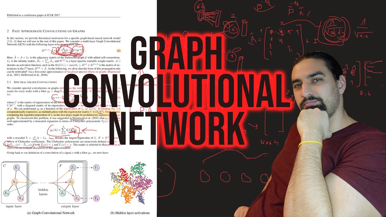
Why this video: This video breaks down the seminal paper on Graph Convolutional Networks (GCNs) by Kipf and Welling. It explains how GCNs use a localized first-order approximation of spectral graph convolutions to pass messages between neighboring nodes without needing expensive eigen-decompositions.

Knowledge Checkpoint:

• Explain why performing an exact eigen-decomposition on the Graph Laplacian is computationally intractable ($O(N^3)$ complexity) for massive web-scale graphs.
• Describe the "renormalization trick" ($A + I$) used in GCNs to prevent exploding or vanishing gradients during node updates.
• Explain how a GCN aggregates features from a node's immediate neighborhood.

---

Why this video: This advanced tutorial contrasts the spectral approach and the spatial approach to graph convolution. It shows how the Graph Fourier Transform (defined by Laplacian eigenvectors) maps graph signals into the frequency domain, where convolutions are computed as pointwise multiplications.

Knowledge Checkpoint:

• Define the Graph Fourier Transform (GFT) of a signal $\mathbf{x}$ using Laplacian eigenvectors.
• Contrast spectral convolutions (which use the spectral properties of the Laplacian) with spatial convolutions (which operate directly on localized node neighborhoods).
• Explain why spectral filters do not naturally generalize to graphs with different structures, and how spatial methods solve this limitation.

---

🔍 Independent Search Challenge (Spectral GCNs & Graph Fourier Transforms)

Because the mathematics of spectral convolutions can be highly abstract, independent study is highly recommended. To deepen your understanding of how deep learning models operate in the graph frequency domain, search for:

"Graph Convolutional Networks spectral vs spatial domain" or "Graph Fourier Transform intuitive explanation spectral graph theory"

Focus on visualizations of how the eigenvectors of the Laplacian serve as "frequencies" (from slowly varying, smooth global patterns to highly oscillating local variations) across a network.

---

Course Map

This flowchart illustrates the logical progression of concepts, showing how you must master basic linear algebra and graph representations before moving on to the Laplacian operator, spectral clustering, and graph-based machine learning applications.

---

Key People Index

As you study this curriculum, you will encounter references to several researchers and historical figures who shaped this field:

• Pierre-Simon Laplace (1749–1827): The French mathematician and physicist who formulated the continuous Laplace operator ($\nabla^2$), which measures the divergence of a gradient. This forms the basis for the discrete Graph Laplacian.
• Miroslav Fiedler (1926–2015): A Czech mathematician whose pioneering work in algebraic graph theory identified the structural significance of the second smallest Laplacian eigenvalue and its corresponding eigenvector (now universally called the Fiedler vector).
• Sergey Brin & Larry Page: The founders of Google, who applied Markov chains and dominant eigenvalues to rank the importance of web pages, creating the PageRank algorithm in 1996.
• Thomas Kipf & Max Welling: Machine learning researchers who developed Graph Convolutional Networks (GCNs) in 2016. They introduced a first-order approximation of spectral filters, making graph-based deep learning computationally scalable.

---

Final Self-Assessment

Test your understanding of the concepts covered in this curriculum with this comprehensive checklist:

• Linear Algebra Foundations: Can you explain why the equation $A\mathbf{x} = \lambda\mathbf{x}$ geometrically means that the vector $\mathbf{x}$ is only scaled, and does not rotate, under the transformation $A$?
• Graph Transformations: Can you construct the Adjacency Matrix ($A$) and Degree Matrix ($D$) for an arbitrary undirected graph with 5 vertices?
• Laplacian Derivation: Can you explain, using the formula $L = D - A$, why multiplying a vector of node values $\mathbf{f}$ by $L$ calculates the difference between a node's value and the average value of its neighbors?
• Boundary Conditions: Do you understand why the unnormalized Laplacian matrix always has a minimum eigenvalue of $\lambda_1 = 0$, and why its corresponding eigenvector is a constant vector ($\mathbf{1}$)?
• Diffusion Mechanics: Can you describe how the eigenvalues of the Graph Laplacian control the rate at which heat or information spreads across a network?
• Algebraic Connectivity: What physical property of a graph does the second smallest eigenvalue ($\lambda_2$) measure, and what does it mean if $\lambda_2 = 0$?
• Spectral Partitioning: Can you describe the steps of using the Fiedler vector to partition a graph into two components?
• Transition vs. Laplacian Dynamics: Can you explain why the PageRank algorithm uses the largest eigenvalue of a transition matrix ($\lambda_1 = 1$), whereas spectral clustering relies on the smallest non-zero eigenvalues of the Laplacian ($\lambda_2, \lambda_3, \dots$)?
• Graph Fourier Transform: Do you understand how the eigenvectors of the Graph Laplacian serve as a Fourier basis, transforming a spatial graph signal into the frequency domain?
• Deep Learning Approximations: Can you explain why modern Graph Convolutional Networks (GCNs) use localized spatial approximations instead of computing exact spectral filters?