IoT Anomaly Detection: Autoencoders & Forests
Learning Goal: Implement and deploy an unsupervised anomaly detection system for industrial IoT sensor data using Autoencoders and Isolation Forests.
Prerequisites
- Basic understanding of programming concepts (variables, loops, and functions).
- High-school level algebra (vectors and matrices).
- Familiarity with basic web concepts (HTTP requests).
Estimated Total Study Time
- Total Estimated Hours: 42 Hours
Module 1: Foundations of Python & Data Handling for IoT
This module builds your baseline technical toolkit. To work with complex Industrial IoT (IIoT) streams, you must first master general Python scripting and learn how to leverage NumPy (for highly efficient numerical operations on multidimensional arrays) and Pandas (to clean, resample, and align time-series data streams).
Recommended Videos

- Why this video: This is the ultimate masterclass for handling raw data using NumPy and Pandas. It provides a structured transition from standard Python environments to the vectorized execution formats essential for big data workloads, showing you how to read CSV files and run descriptive statistics.

- Why this video: Industrial IoT data is fundamentally time-series data. This step-by-step tutorial teaches you how to index dataframes by timestamps, extract hourly or daily trends, run datetime logic, and filter time ranges with high performance.

- Why this video: An essential follow-up that details the nuances of Pandas datetime formats and timestamps. You will learn to parse dates, convert string series to actual date indices, and manage timezone-aware readings.
Knowledge Checkpoint
- Convert a dataframe's index to a DatetimeIndex using
pd.to_datetime(). - Resample raw timestamped sensor readings to consistent 1-minute averages.
- Explain why NumPy operations run significantly faster than standard Python lists.
- Handle timezone changes and localize raw UTC timestamp data.
Module 2: Industrial IoT & Anomaly Detection Concepts
Industrial IoT (IIoT) sensors are bound by physics, working under high-stress operating conditions. Consequently, they introduce heavy noise, missing signals, and dropouts. This module covers physical concepts of IIoT telemetry, outlines what constitutes an unsupervised "anomaly," and details how to preprocess, clean, and align raw sensor signals.
Gap Note: While the video pool has high-quality sensor cleaning tutorials, general IIoT business lectures can lack depth on physical mathematical formulas. If you want a deeper theoretical dive, independently search for: "Industrial sensor data preprocessing and cleaning Python".
Recommended Videos

- Why this video: Explains why industrial applications require higher standards of precision, reliability, and security than typical consumer smart devices. It contextualizes the physical environments where your algorithms will operate.
- Why this video: This presentation provides a highly technical, real-world framework for cleaning raw sensor logs. It details handling missing signals, resolving duplications, interpolating signal loss, and stripping systemic outliers.

- Why this video: Crucial for setting up inputs for multi-dimensional anomaly pipelines. Shows how to use shifted logs, compute rolling offsets, construct lag features, and preprocess raw timespan records into matrices.

- Why this video: Introduces the mathematical necessity of sensor alignment, axis mapping, and noise cancellation. Though focused on software filters, the structural steps apply directly to cleaning noisy ML features.
Knowledge Checkpoint
- Define the primary differences between Consumer IoT and Industrial IoT constraints.
- Use
pandas.DataFrame.shift()to construct lag variables for multi-step predictions. - Differentiate between sudden anomalous spikes (point anomalies) and prolonged, drifting deviations (contextual/collective anomalies).
- Select appropriate imputation strategies (e.g., forward-fill, linear interpolation) for broken sensor periods.
Module 3: Isolation Forests for Anomaly Detection
Isolation Forest is a highly effective machine learning algorithm for tabular and multi-dimensional anomaly detection. Unlike traditional techniques that construct profiles of normal points, Isolation Forests isolate anomalies by recursively partitioning data space. This module covers the math, structure, and implementation of this tree-based outlier model.
Gap Note: While the videos below cover standard Scikit-Learn implementations and basic properties, they lack high-end visual animations of vector partitioning. For a deeper visualization of space splits, search for: "Isolation Forest algorithm machine learning math explained".
Recommended Videos
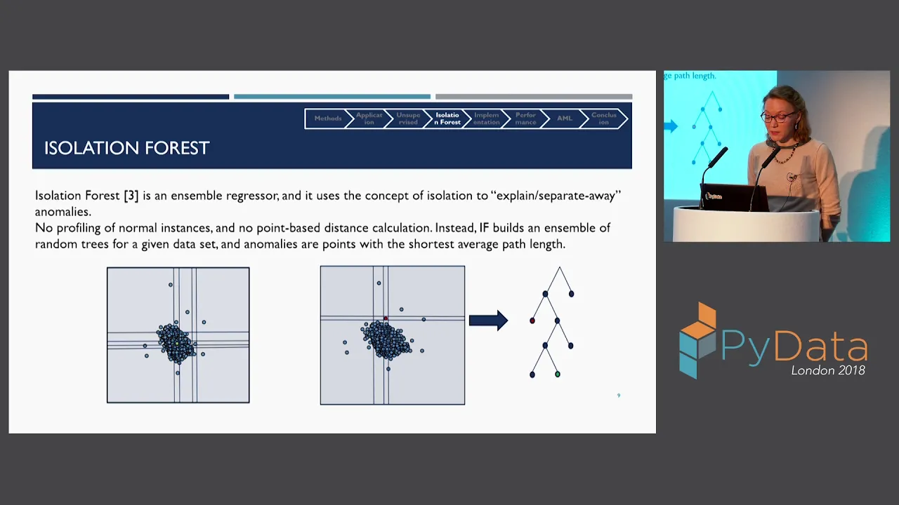
- Why this video: A clear mathematical and structural introduction showing why isolation-based models outperform distance and density estimators on high-dimensional data.
- Why this video: Explains the core mechanism of tree partition paths: how random binary splitting isolates spatial anomalies rapidly (resulting in short tree paths) compared to clustered nominal observations.

- Why this video: A hands-on tutorial that shows you how to initialize
IsolationForestin Scikit-Learn, setcontamination levels, train models, and extract anomaly scores.
Knowledge Checkpoint
- Explain why anomalies require fewer random spatial partitions to isolate than normal points.
- Define the role of the
contaminationparameter in Scikit-Learn'sIsolationForest. - Describe how the average path length () of isolation trees maps to an anomaly score .
- Implement
model.fit()andmodel.predict()to return outlier labels (-1 for anomalies, 1 for normal).
Module 4: Deep Learning & Autoencoders for Anomalies
Autoencoders use neural networks to perform unsupervised reconstruction. By bottlenecking data through low-dimensional layers, the network learns to reconstruct normal, highly correlated sensor characteristics. When presented with anomalous patterns, the network struggles to reconstruct them properly, resulting in high reconstruction error.
Recommended Videos

- Why this video: The gold standard for understanding neural networks. This video details how matrices, weights, biases, and activation functions work together to process input signals.
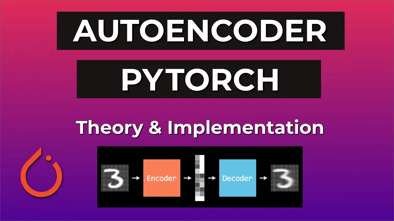
- Why this video: A practical PyTorch-specific tutorial. You will learn to construct custom
EncoderandDecoderclasses, pass vectors through a latent bottleneck, write optimization loops, and calculate loss.
- Why this video: Shows you how to design a specialized temporal autoencoder for sensor arrays. This tutorial covers handling sequence formats in PyTorch, reconstructing structured signals, and isolating deviations via Mean Squared Error (MSE) thresholds.
Knowledge Checkpoint
- Sketch the core architecture of an Autoencoder (Input Layer Bottleneck/Latent Space Output Layer).
- Write a custom PyTorch model subclassing
nn.Modulecontaining encoder linear units and decoder units. - Explain why the network fails to reconstruct anomalies if it is only trained on nominal data.
- Calculate the reconstruction loss metric using PyTorch's
nn.MSELoss.
Module 5: System Integration & Evaluation Metrics
This module integrates your classical ML model (Isolation Forest) and your deep learning system (Autoencoder). Because unsupervised problems lack ground-truth validation labels, we must use alternative validation strategies: training on clean normal periods (semi-supervised), injecting synthetic outliers, and tracking statistical deviations.
Gap Note: Video tutorials on combining models into voting ensembles are scarce. To research this concept further, look for: "Unsupervised anomaly detection evaluation metrics and validation".
Recommended Videos

- Why this video: Explains why typical supervised classifiers fall flat on sparse real-world anomaly data and provides systemic advice on structuring unsupervised validation pipelines.

- Why this video: Explains how to evaluate highly imbalanced data. It details the math behind Precision, Recall, and F1-Score, showing how to balance false positives and false negatives.

- Why this video: A concise overview of model validation best practices. It highlights key differences in evaluation strategies when labels are sparse versus entirely absent.
Pragmatic Validation & Integration Strategies
        +------------------------------------+
        | Raw IIoT Sensor Stream (Multivariate)|
        +-----------------+------------------+
                          |
                 +--------+--------+
                 |                 |
                 v                 v
         +---------------+ +---------------+
         | Autoencoder   | | Isolation     |
         | Model (MSE)   | | Forest (Score)|
         +-------+-------+ +-------+-------+
                 |                 |
                 | Reconst. Error  | Outlier Label
                 v                 v
        +------------------------------------+
        | Weighted Voting / Ensemble Decision|
        +-----------------+------------------+
                          |
                          v
              Final Anomalous Event?
              [Yes (Trigger) / No]
1. Statistical Threshold Calibration
Instead of arbitrarily setting reconstruction error limits, set your anomaly thresholds based on statistical distributions.
- Calculate Mean Squared Error (MSE) across a known, healthy validation partition.
- Set your trigger threshold () using the validation mean () and standard deviation (): This ensures that normal data variance only triggers false alarms of the time.
2. Synthetic Outlier Injection
When true labels are missing, you can evaluate model sensitivity by injecting artificial anomalies into your validation sets:
- Spike Injection: Add sudden random offsets () to individual sensor columns.
- Drift Injection: Gradually add a linear trend line to simulate sensor degradation.
- Signal Loss: Replace segments of your validation data with a flat constant line (frozen sensor).
- Measure your model's recall against these injected events to evaluate its real-world effectiveness.
3. Classical & Deep Learning Ensembles
Combine the strengths of your models using a simple voting ensemble:
- Feature Extraction: Pass input data through your Autoencoder and extract the reconstruction error as a new feature.
- Forest Injection: Pass your original features plus this reconstruction error feature into the Isolation Forest.
- This hybrid approach leverages both spatial partitioning (Isolation Forest) and reconstruction capacity (Autoencoder).
Knowledge Checkpoint
- Define why classical accuracy is a misleading metric for highly imbalanced anomaly sets.
- Implement threshold boundaries based on validation data standard deviation ().
- Inject synthetic spikes or drift to evaluate model sensitivity.
- Design an ensemble that triggers an alert only when both models exceed their confidence limits.
Module 6: Deploying IoT ML Models to Production
To deliver real business value, anomaly detection models must run close to the data source. This module covers wrapping your trained PyTorch and Scikit-Learn pipelines in high-performance FastAPI endpoints and streaming raw sensor arrays through an event-driven Apache Kafka pipeline.
Recommended Videos

- Why this video: Shows you how to serve Python models over HTTP using FastAPI. You will learn how to design POST endpoints, accept JSON payloads, parse inputs, and return prediction dicts.

- Why this video: Takes your local web server and prepares it for production. It covers building lightweight Docker files, containerizing dependencies, and managing environment parameters.

- Why this video: A great hands-on guide for streaming applications. It teaches you how to spin up Apache Kafka brokers, configure publishers/consumers in Python, and process streaming messages.
Knowledge Checkpoint
- Build a FastAPI server with a
/predictendpoint that accepts sensor values as JSON. - Write a Dockerfile to package your model, endpoints, and PyTorch dependencies.
- Run a Python Kafka consumer that reads sensor streams and passes payloads to your model in real time.
- Minimize endpoint latency by serving predictions using pre-loaded model states.
Course Map
Below is the recommended path through the course. You must complete the data engineering foundations (Modules 1 and 2) before starting the core machine learning tracks.
Key People Index
- Fei Tony Liu, Ting Kai Ming, and Zhou Zhi-Hua: The computer scientists who pioneered the Isolation Forest algorithm (2008), shifting the anomaly detection paradigm from profiling normal points to explicitly isolating anomalies.
- Grant Sanderson (@3blue1brown): An educator acclaimed for visual explanations of complex mathematics. His linear algebra and neural network visual series form the mathematical foundation for Module 4.
- Elena Sharova: A seasoned data scientist and author who champions open-source tools for tree-based anomaly detection. Her PyData presentations make complex algorithms accessible.
Final Self-Assessment
Complete these tasks to verify you have met the learning goals of the curriculum:
- Clean a raw, noisy sensor log file containing missing values and timestamps using Pandas.
- Resample multiple sensors with varying sampling rates into an aligned 1-second interval dataframe.
- Train a Scikit-Learn
IsolationForeston your tabular sensor data and extract anomaly labels. - Write a custom PyTorch Autoencoder containing fully connected layers and a narrow bottleneck.
- Train the Autoencoder on healthy normal sequences and verify that reconstruction error decreases during training.
- Calibrate an anomaly threshold () using the statistical distribution of normal validation reconstruction errors.
- Inject synthetic anomalies (spikes and drifts) into a clean validation dataset and measure your model's Precision, Recall, and F1-score.
- Build a FastAPI web server that loads your trained models and runs real-time inference.
- Containerize your FastAPI application using Docker.
- Connect a Python Kafka consumer to stream simulated sensor payloads into your containerized inference API.