Building Ray Tracers: C++ & Linear Algebra

Learning Goal: Build a high-performance 3D software ray tracer from first principles using C++ and linear algebra. By the end of this course, you will understand how to set up a clean C++ build environment, mathematically model vector spaces, project rays from a virtual camera, compute intersections with geometric primitives, simulate physically based materials (Lambertian, metallic, and glass/dielectrics), and optimize execution speeds using multi-threading and hierarchical spatial partitioning (BVH).

Prerequisites

• Basic familiarity with programming logic (variables, loops, and conditional statements in any language).
• High-school level algebra and trigonometry. No prior multi-variable calculus or advanced physics is required.

Course Metadata

• Estimated Total Study Time: 35 Hours
• Course Format: Video-assisted, project-based self-study with focus on raw implementation from scratch.

---

Module 1: C++ Programming Fundamentals for Graphics

This module bridges the gap for beginners and transition-programmers to C++ by establishing a rock-solid dev setup and explaining high-performance low-level systems programming concepts. You will study compiling, memory organization, and object instantiation—critical concepts for low-overhead graphics computing.

Why this video: High-performance graphics applications require a deep understanding of your build ecosystem. Dr. Mike Shah breaks down how C++ source files go from human-readable text down to preprocessed, compiled, assembled, and linked binaries, enabling you to debug linker errors when building your software ray tracer.

Why this video: Establishing a clean compiler path is often the hardest part of C++ development. This step-by-step guide helps you install the MinGW compiler suite, configure Windows environment variables, and verify that your system can run the g++ compiler from command lines.

Why this video: Pointers are infamous but crucial for spatial acceleration data structures. Javidx9 provides an exhaustive, highly visual animation of memory address spaces, references, pointers, dereferencing, and the physical reality of RAM.

Why this video: Knowing when to instantiate objects on the Stack versus the Heap determines your renderer's speed. The Cherno explains the performance trade-offs, showing how stack instantiation avoids system-level allocations while heap allocation handles dynamic life cycles.

Knowledge Checkpoint

• Understand the role of headers (.h/.hpp) vs implementation files (.cpp) and what happens during the Linking phase.
• Successfully run g++ -std=c++17 main.cpp -o raytracer inside your terminal of choice.
• Trace memory addresses and draw diagrams of pointers referencing variables on the heap/stack.
• Differentiate between Stack Allocation (Vector3 v;) and Heap Allocation (Vector3* v = new Vector3();) and explain the cache performance benefits of the stack.

---

Module 2: Vector Math & Linear Algebra Foundations

Ray tracing is pure linear algebra in action. In this module, you will master vectors, coordinate systems, linear combinations, coordinate transforms, and basic trigonometry—all translated directly into code.

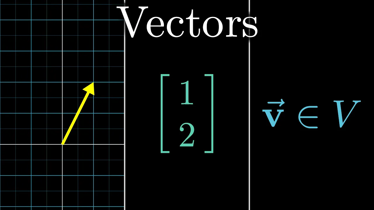
Why this video: Grant Sanderson provides the best intuitive, visual understanding of vectors from physics, computer science, and mathematical perspectives. This is critical for conceptualizing coordinates inside virtual space.

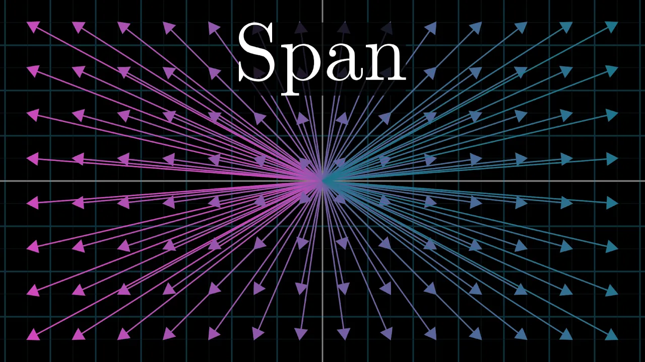
Why this video: Under the hood, camera coordinate systems and ray directions are built upon basis vectors. This video explains how scaling and adding basis vectors spans the 3D rendering canvas.

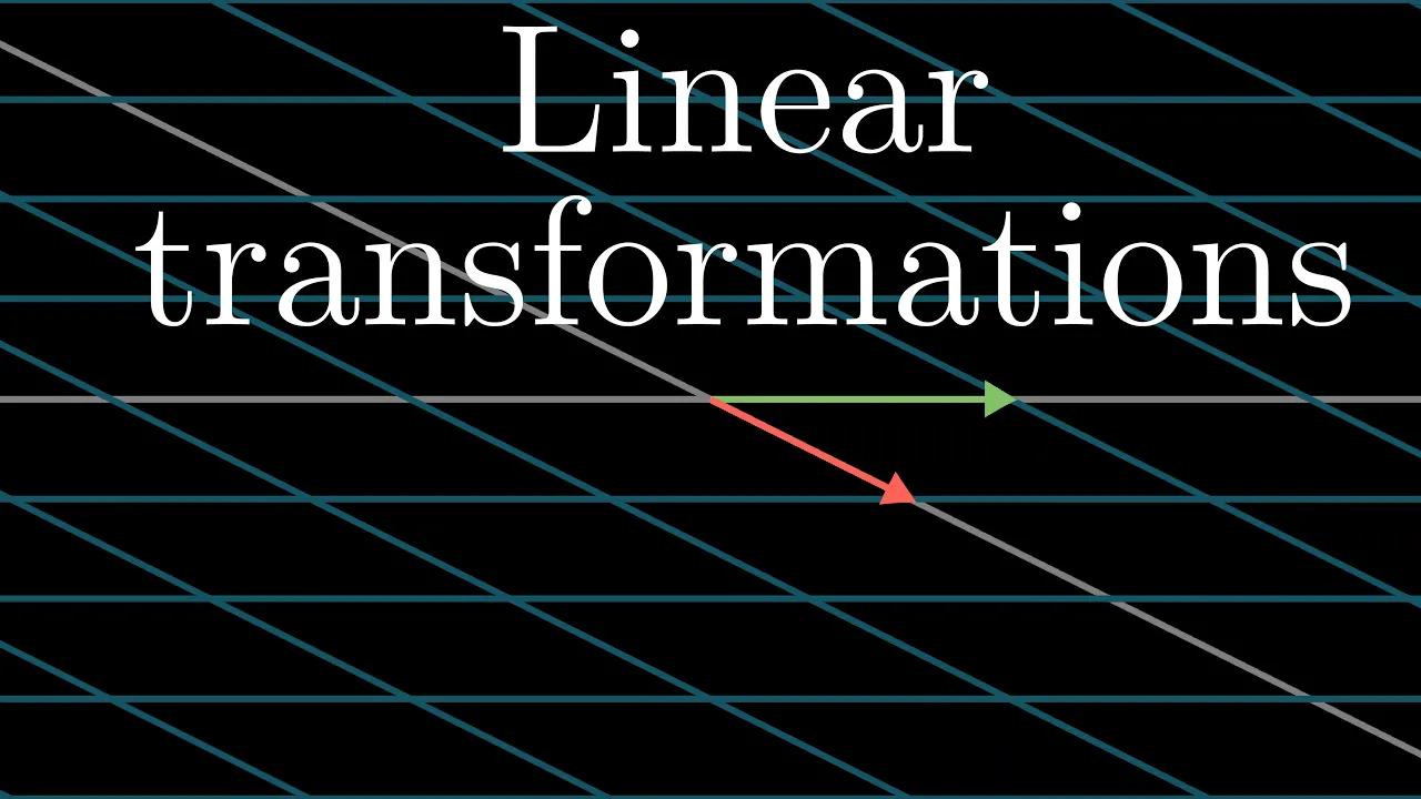
Why this video: Moving, rotating, and scaling objects in 3D scenes relies on matrices. This chapter visualizes matrices as "coordinate manipulations," giving you an intuitive grasp of transformations before you write your matrix classes.

Why this video: Freya Holmér presents the math with direct game-engine focus. This segment bridges pure mathematical theory into vector operations like additions, subtractions, magnitude calculations, and vector normalizing.

Knowledge Checkpoint

• Define what a unit vector is and write C++ logic to normalize any arbitrary Vector3 struct.
• Program dot product ($A \cdot B$) and cross product ($A \times B$) functions in your own custom vector library.
• Describe the physical/geometric meaning of a zero, positive, or negative dot product result.
• Mentally trace how matrix-vector multiplication transforms coordinates from world space to object space.

---

Module 3: Camera Modeling & Ray-Sphere Intersection

Now, the core loop begins. In this module, you will define the parametric mathematical equation of a 3D ray and derive the quadratic system that calculates whether a ray pierces a sphere.

Why this video: Prof. Solomon introduces the foundational rendering equation and shows how a ray is defined mathematically as a parametric function $P(t) = O + tD$.

Why this video: This is a compact, code-focused video illustrating the execution of ray-sphere mathematical intersections. It shows how the quadratic equation is solved in real C++ code to draw a basic colored circle on screen.

Why this video: This video offers a great high-level conceptual walkthrough of rendering scenes pixel-by-pixel, explaining how the screen relates to a 2D image plane mapped in front of a 3D eye.

🔍 Identified Gap: Detailed Camera Coordinate Mapping

The video pool lacks granular math derivation on converting raw screen pixels $(x, y)$ coordinates (from $0$ to $Width$, and $0$ to $Height$) into normalized viewport coordinates, and finally mapping those to a 3D ray direction in world space.

Independent Study Guide & Recommended Search Query:

• Search Query: Ray generation camera viewport math C++ ray tracer
• Core Logic to Implement: To generate a ray for pixel $(i, j)$:
  1. Calculate normalized screen coordinates: $u = \frac{i + \delta}{Width - 1}$, $v = \frac{j + \delta}{Height - 1}$ (where $\delta$ is an offset, typically $0.5$ for center, or randomized for anti-aliasing).
  2. Given a field of view (FOV) and Aspect Ratio ($AR$), find the viewport boundaries: $Height_{vp} = 2 \cdot \tan\left(\frac{FOV}{2}\right)$ $Width_{vp} = AR \cdot Height_{vp}$
  3. Construct camera coordinate frame using standard basis vectors $u, v, w$ computed from camera position (lookfrom), target (lookat), and world-up vector.

Knowledge Checkpoint

• Implement the Ray class structure: struct Ray { Vec3 origin; Vec3 direction; };
• Solve the algebraic quadratic equations for sphere intersection: $at^2 + bt + c = 0$, where: $a = \mathbf{d} \cdot \mathbf{d}$ $b = 2\mathbf{d} \cdot (\mathbf{o} - \mathbf{c})$ $c = (\mathbf{o} - \mathbf{c}) \cdot (\mathbf{o} - \mathbf{c}) - r^2$
• Successfully output a static image file format (such as .ppm or .png) displaying a 3D sphere suspended in space.

---

Module 4: Lighting, Surface Normals, and Anti-Aliasing

Static colors look flat. To make shapes look round and dynamic, you must calculate surface normals, handle light reflections using the Lambertian diffuse model, use recursive calls for light bounces, and implement stochastic anti-aliasing to eliminate jagged edges.

Why this video: This video derives Lambert’s Cosine Law, demonstrating how the angle between the incoming light vector and the surface normal determines lighting intensity.

Why this video: This practical video guides you through implementing anti-aliasing. By casting multiple slightly randomized rays per pixel (supersampling) and averaging their colors, your renderer transitions from harsh, jagged blockiness to smooth edges.

Why this video: Legendary programmer John Carmack discusses light behavior, reflections, and computational approximations of diffuse and specular surfaces. This bridges mathematical approximations with the physical reality of photons.

Knowledge Checkpoint

• Calculate the surface normal vector at any intersection point $P$ on a sphere with center $C$ using: $\mathbf{N} = \frac{\mathbf{P} - \mathbf{C}}{r}$
• Implement diffuse reflection by bouncing secondary rays inside a hemisphere surrounding the surface normal vector (using random unit vectors).
• Program a recursive depth-limiting loop to handle multiple light bounces, returning background sky color when depth reaches zero.
• Build a multi-sample grid helper that draws and averages 10–100 sub-pixel samples for anti-aliasing.

---

Module 5: Advanced Materials: Metal & Glass

Perfect spheres with flat colors are not enough. This module details specular reflections for metals, refractive transparency based on Snell's Law for glass, and Fresnel reflectivity calculations.

Why this video: Freya Holmér derives vector reflection math visually. You will directly use this formula, $\mathbf{R} = \mathbf{V} - 2(\mathbf{V} \cdot \mathbf{N})\mathbf{N}$, to write metallic reflection code.

Why this video: Sebastian Lague explains the mechanics of transparency, showing how light refracts (bends) when crossing interfaces of air, glass, and water. He covers refraction, total internal reflection, and refraction indices.

🔍 Identified Gap: Dielectric & Refraction Implementations in Raw C++

Most visual engine-level guides rely on pre-built shaders or node graphs. Your software ray tracer requires implementing raw C++ vector math routines for Snell's Law and Fresnel reflection coefficients.

Independent Study Guide & Recommended Search Query:

• Search Query: Snell's law refraction vector derivation computer graphics
• Mathematical Reference for Refraction Vector $\mathbf{T}$: Given unit incoming ray vector $\mathbf{I}$, unit surface normal $\mathbf{N}$, and refractive index ratio $\eta = \frac{\eta_1}{\eta_2}$: $\cos\theta_1 = -\mathbf{N} \cdot \mathbf{I}$ $\sin^2\theta_2 = \eta^2(1 - \cos^2\theta_1)$ If $\sin^2\theta_2 > 1.0$, Total Internal Reflection (TIR) occurs; light cannot refract and must reflect instead. Otherwise, the refracted direction is: $\mathbf{T} = \eta\mathbf{I} + \left(\eta\cos\theta_1 - \sqrt{1 - \sin^2\theta_2}\right)\mathbf{N}$
• Schlick's Approximation for Fresnel Reflectivity $R(\theta)$: $R_0 = \left(\frac{\eta_1 - \eta_2}{\eta_1 + \eta_2}\right)^2$ $R(\theta) = R_0 + (1 - R_0)(1 - \cos\theta)^5$

// Pure C++ implementation skeleton struct Material { virtual bool scatter(const Ray& r_in, const HitRecord& rec, Color& attenuation, Ray& scattered) const = 0; };

class Dielectric : public Material { public: double ir; // Index of Refraction Dielectric(double index_of_refraction) : ir(index_of_refraction) {}

virtual bool scatter(const Ray& r_in, const HitRecord& rec, Color& attenuation, Ray& scattered) const override { attenuation = Color(1.0, 1.0, 1.0); double refraction_ratio = rec.front_face ? (1.0 / ir) : ir; Vec3 unit_direction = unit_vector(r_in.direction()); double cos_theta = fmin(dot(-unit_direction, rec.normal), 1.0); double sin_theta = sqrt(1.0 - cos_theta*cos_theta); bool cannot_refract = refraction_ratio * sin_theta > 1.0; Vec3 direction; if (cannot_refract || reflectance(cos_theta, refraction_ratio) > random_double()) { direction = reflect(unit_direction, rec.normal); } else { direction = refract(unit_direction, rec.normal, refraction_ratio); } scattered = Ray(rec.p, direction); return true; }

private: static double reflectance(double cosine, double ref_idx) { // Schlick's approximation auto r0 = (1-ref_idx) / (1+ref_idx); r0 = r0*r0; return r0 + (1-r0)*pow((1 - cosine), 5); } };

Knowledge Checkpoint

• Program a metallic material class that reflects rays perfectly and includes a customizable fuzz parameter to simulate rough metal surfaces.
• Mathematically derive Snell's Law and program a robust vector refraction function.
• Integrate Schlick's approximation so that glass spheres appear more reflective at steep grazing angles.

---

Module 6: Optimization Part I - Multi-Threading

With anti-aliasing and recursive bouncing active, your renderer will slow down drastically. Because each pixel can be computed independently of all other pixels, ray tracing is an "embarrassingly parallel" problem. This module covers leveraging multiple CPU cores to scale performance.

Why this video: The Cherno demonstrates practical strategies to multi-thread a software renderer in C++. He discusses dividing screen buffers into smaller work units and allocating thread tasks to maximize hardware utilization.

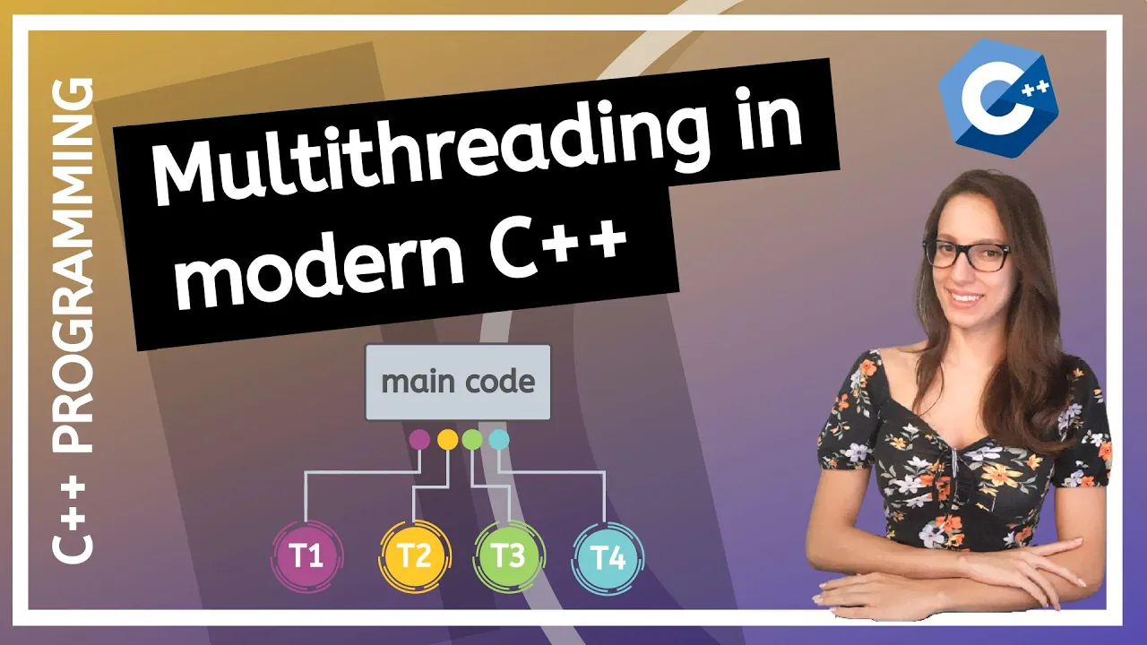
Why this video: A clear introduction to threading fundamentals in standard modern C++. You'll learn how to instantiate, manage, and synchronize std::thread workers without causing race conditions or deadlocks.

🔍 Identified Gap: Pixel Loop Multi-threading in C++

Applying general-purpose threading primitives directly into nested performance-sensitive rendering loops requires specific patterns.

Independent Study Guide & Recommended Search Query:

• Search Query: Multi-threading ray tracer C++ std thread openmp
• Implementation Strategies:
  1. Standard Library Parallelism (C++17): Use std::for_each combined with standard execution policies.

     #include <execution>
     #include <vector>
     
     std::vector<int> image_rows(height);
     // Populate row indices
     std::iota(image_rows.begin(), image_rows.end(), 0);
     
     std::for_each(std::execution::par, image_rows.begin(), image_rows.end(), [width](int y) {
         for (int x = 0; x < width; ++x) {
              // Calculate pixel colors in parallel...
         }
     });
     

  2. OpenMP: An alternative and highly cross-platform way to parallelize loops using simple compiler pragmas.

     #pragma omp parallel for schedule(dynamic)
     for (int y = 0; y < height; ++y) {
         for (int x = 0; x < width; ++x) {
             // Calculate pixel colors in parallel...
         }
     }
     

Knowledge Checkpoint

• Spawn multiple std::thread instances, slice your coordinate system into linear horizontal segments, and distribute them to render asynchronously.
• Prevent race conditions by ensuring threads write exclusively to independent memory slots in a pre-allocated pixel buffer.
• Measure rendering times to verify that doubling active CPU thread workers yields near-linear execution scaling.

---

Module 7: Optimization Part II - Acceleration Structures (BVH)

Even with many CPU cores, checking every ray against thousands of polygons or spheres is incredibly slow, running at $O(N)$ time complexity. This module teaches you how to construct a Bounding Volume Hierarchy (BVH) to lower intersection calculations to $O(\log N)$ logarithmic complexity.

Why this video: James Lambert presents an exceptionally clear spatial visualization of Bounding Volume Hierarchies (BVH). He shows how grouping spatial geometry into nested, overlapping boxes allows renderers to skip checking huge clusters of geometry with a single ray-box intersection test.

Why this video: This video introduces the specialized hardware acceleration structures utilized by modern GPUs. It explains why BVH is the absolute standard across industrial graphics pipelines and the physical hardware level.

🔍 Identified Gap: C++ Implementation of a BVH Tree Node

The video pool introduces the concepts of BVH, but lacks a code implementation showing how to split nodes and recursively traverse a bounding volume tree structure.

Independent Study Guide & Recommended Search Query:

• Search Query: Bounding Volume Hierarchy BVH ray tracing implementation C++
• Implementation Plan:
  1. Define an Axis-Aligned Bounding Box class (AABB), which holds two coordinate bounds: minimum and maximum.
  2. Implement a quick AABB::hit(const Ray& r, double t_min, double t_max) intersection function (often using Andrew Kensler's fast AABB intersection algorithm).
  3. Construct a BVHNode class that inherits from your general Hitable base class:

     class BVHNode : public Hitable {
     public:
         std::shared_ptr<Hitable> left;
         std::shared_ptr<Hitable> right;
         AABB box;
     
         BVHNode(const std::vector<std::shared_ptr<Hitable>>& src_objects, size_t start, size_t end) {
             auto objects = src_objects; // Modifiable copy
             int axis = random_int(0, 2); // Split along a random axis (X, Y, or Z)
             
             // Sort primitives along the chosen axis
             auto comparator = (axis == 0) ? box_x_compare
                             : (axis == 1) ? box_y_compare
                             : box_z_compare;
     
             size_t object_span = end - start;
             if (object_span == 1) {
                 left = right = objects[start];
             } else if (object_span == 2) {
                 if (comparator(objects[start], objects[start+1])) {
                     left = objects[start];
                     right = objects[start+1];
                 } else {
                     left = objects[start+1];
                     right = objects[start];
                 }
             } else {
                 std::sort(objects.begin() + start, objects.begin() + end, comparator);
                 auto mid = start + object_span/2;
                 left = std::make_shared<BVHNode>(objects, start, mid);
                 right = std::make_shared<BVHNode>(mid, end);
             }
             
             AABB box_left, box_right;
             left->bounding_box(box_left);
             right->bounding_box(box_right);
             box = surrounding_box(box_left, box_right);
         }
     
         virtual bool hit(const Ray& r, double t_min, double t_max, HitRecord& rec) const override {
             if (!box.hit(r, t_min, t_max)) return false;
             
             bool hit_left  = left->hit(r, t_min, t_max, rec);
             bool hit_right = right->hit(r, t_min, hit_left ? rec.t : t_max, rec);
             
             return hit_left || hit_right;
         }
     };
     

Knowledge Checkpoint

• Program an Axis-Aligned Bounding Box (AABB) intersection calculator.
• Implement a node-sorting build pass that groups shapes along spatial dimensions (X, Y, or Z).
• Build a recursive tree-traversal routine that skips searching half of your 3D objects if their bounding box isn't intersected.
• Test scene performance with 10,000 randomized spheres, demonstrating an order of magnitude rendering speed increase.

---

Course Map

---

Key People Index

• Bjarne Stroustrup: Creator of the C++ language. His initial vision of combining object-oriented modularity with low-level memory control forms the foundation of modern high-performance graphics engine architectures.
• Grant Sanderson: Educator behind the YouTube channel 3Blue1Brown. His visual geometric intuition of linear transformations has helped thousands of computer graphics engineers build clean 3D coordinate mapping systems.
• John Carmack: Pioneer of real-time computer graphics, co-founder of id Software, and Lead Developer of Doom and Quake. His insights on performance optimizations, math simplifications, and light physics models remain essential references for game developers worldwide.
• Peter Shirley: Renowned graphics researcher and author of the famous "Ray Tracing in One Weekend" series. His educational methodologies helped standardize the modern approach of teaching ray tracers sequentially from first principles.

---

Final Self-Assessment

Complete this comprehensive self-assessment to certify that your home-grown ray tracer is mathematically and programmatically correct.

• Build Check: Your project compiles natively under an optimized release flag (-O3) without yielding errors or dangling pointers.
• Vector Precision: Your custom vector mathematical operations (dot products, cross products, reflections, and refractions) produce accurate outputs in unit-tests.
• Perspective Mapping: Your camera produces correct field of view (FOV) changes and supports custom coordinate offsets for look-at and up orientation.
• Diffuse Realism: Your diffuse surfaces match Lambertian cosine falloffs (surfaces are brightest when facing the light direction perpendicularly).
• Specular Metals: Your metallic materials support reflections, fuzz indices, and do not lose energy during bounces.
• Snell's Law Glass: Your dielectric materials handle internal refraction, total internal reflection, and use Schlick's approximation to model realistic grazing angle reflections.
• Multi-threaded CPU: Your program utilizes all active CPU cores, rendering scenes faster than a single-threaded execution loop.
• Logarithmic BVH Speed: Your renderer can run scenes containing more than 10,000 geometric shapes inside reasonable rendering windows, confirming a functional spatial partitioning tree structure ($O(\log N)$).