Fourier Transform: Series, Calculus & DSP

Learning Goal: Mastering the Fourier Transform: Understanding the mathematical journey from basic trigonometric series to discrete signal processing applications.

• Prerequisites: High-school algebra, trigonometry, and basic single-variable calculus (derivatives and integration).
• Estimated Study Time: 16 Hours

Module 1: Mathematical Foundations: Complex Numbers & Waves

This module establishes the essential mathematical building blocks. You will explore how complex numbers, polar coordinates, and Euler's formula combine to represent rotating vectors (phasors) in the complex plane, which serves as the geometric language of the Fourier Transform.

Recommended Videos

Introduction to Complex Numbers: Lecture 2 - Oxford Mathematics 1st Year Student Lecture

@OxfordMathematics03:122477818

Introduction to Complex Numbers: Lecture 2 - Oxford Mathematics 1st Year Student Lecture

Euler's formula states e^(iθ) = cosθ + i sinθ for real θ. This enables compact exponential representation: if z has modulus R and argument θ, then z = Re^(iθ). This notation simplifies multiplication (multiply moduli, add exponents) and is particularly useful for roots and powers. The exponential form connects complex analysis with calculus and differential equations.

@OxfordMathematics · 03:12

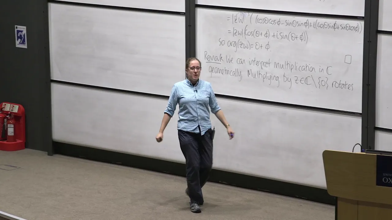
• Why this video: This lecture segment provides an elegant, rigorous introduction to Euler's formula from one of the world's leading academic institutions. It demonstrates the compact exponential notation $z = Re^{i\theta}$, setting up the geometric foundations of rotating vectors (phasors).
• Knowledge checkpoint:
  • State Euler's formula and identify its components ($R$, $e$, $i$, $\theta$).
  • Convert a complex number from rectangular form ($a+bi$) to polar/exponential form ($Re^{i\theta}$).
  • Explain how multiplying complex exponentials affects their magnitude and phase angle.

Euler's formula with introductory group theory

@3blue1brown24:282652263

Euler's formula with introductory group theory

Euler's formula e^(πi) = -1 can be understood through group theory by recognizing that the exponential function maps the additive group of complex numbers (vertical translations) to the multiplicative group of complex numbers (rotations), with the special base e ensuring that a vertical translation of π units corresponds to a rotation of exactly π radians (180 degrees), which geometrically represents the number -1.

@3blue1brown · 24:28

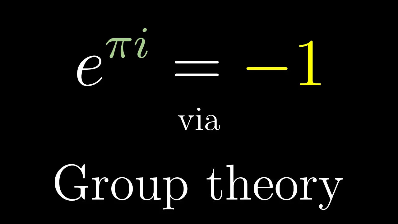
• Why this video: Visualizing mathematics is key to deep intuition. Grant Sanderson explains Euler's formula conceptually, using group theory to map the additive group of complex numbers (vertical movements/translations) to the multiplicative group of the complex plane (rotations).
• Knowledge checkpoint:
  • Visualize $e^{i\theta}$ as a path tracing the unit circle in the complex plane.
  • Describe how the exponential function acts as a mapping from linear/vertical additions to circular rotations.
  • Explain how the derivative of $e^{it}$ with respect to $t$ is always perpendicular to its position vector, implying uniform circular motion.

Complex Numbers and Euler's Formula \| MIT 18.03SC Differential Equations, Fall 2011

@mitocw11:30170820

Complex Numbers and Euler's Formula \| MIT 18.03SC Differential Equations, Fall 2011

Complex numbers can be represented in rectangular form (a + ib) or polar form (r × e^(iθ)), where r is the modulus (√(a² + b²)) and θ is the phase angle (tan⁻¹(b/a)), with Euler's formula e^(iθ) = cos(θ) + i sin(θ) enabling conversion between these representations; this framework allows computation of complex operations like reciprocals and roots through manipulation of modulus and phase rather than direct algebraic manipulation.

@mitocw · 11:30

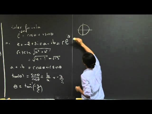
• Why this video: A foundational lecture that bridges abstract complex arithmetic with practical differential equations and engineering mathematics. It provides the essential algebraic drills to ensure you can confidently manipulate complex exponents.
• Knowledge checkpoint:
  • Compute the modulus $r = \sqrt{a^2 + b^2}$ and argument $\theta = \tan^{-1}(b/a)$ of any complex coordinates.
  • Divide two complex numbers by multiplying the numerator and denominator by the complex conjugate.
  • Transition seamlessly between rectangular coordinates ($a + ib$) and polar representations ($re^{i\theta}$).

Module 2: The Fourier Series: Decomposing Periodic Signals

Here, you will transition from individual waves to signal decompositions. This module covers how any periodic signal can be represented as an infinite sum of simple sine and cosine waves (or complex exponentials), introducing the core concept of the frequency domain.

Review Note on Mathematical Gaps: While the videos below offer incredible insight, our video pool lacks a highly-rated step-by-step math derivation starting from basic trigonometric orthogonal projection. To supplement this, pay special attention to the Oxford Calculus derivation video, which walks through this process in detail.

Recommended Videos

Oxford Calculus: Fourier Series Derivation

@TomRocksMaths41:1770743

Oxford Calculus: Fourier Series Derivation

Fourier Series coefficients for a 2L-periodic function f(x) are derived using orthogonality relations: the constant term a₀ = (1/L)∫₋ᴸᴸ f(x)dx, the cosine coefficients aₙ = (1/L)∫₋ᴸᴸ f(x)cos(nπx/L)dx, and the sine coefficients bₙ = (1/L)∫₋ᴸᴸ f(x)sin(nπx/L)dx, where the orthogonality of sine and cosine functions ensures that cross terms vanish when integrating over the symmetric interval [-L, L].

@TomRocksMaths · 41:17

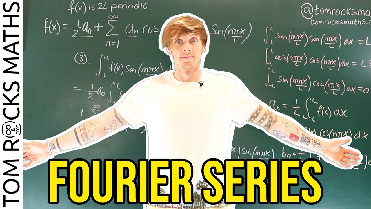
• Why this video: This long-form, rigorous video specifically plugs the mathematical derivation gap. It takes you step-by-step through the derivation of Fourier coefficients ($a_0, a_n, b_n$) using the orthogonality relations of sine and cosine functions.
• Knowledge checkpoint:
  • Explain why the integral of $\sin(nx)\cos(mx)$ over a symmetric interval $[-\pi, \pi]$ equals zero (orthogonality).
  • Mathematically derive the expression for $a_0$, $a_n$, and $b_n$ by integrating the projection of $f(x)$ onto trigonometric basis functions.
  • Explain how orthogonality acts like a "sieve" to isolate individual frequency components from a compound periodic wave.

Intro to FOURIER SERIES: The Big Idea

@DrTrefor10:44387023

Intro to FOURIER SERIES: The Big Idea

A Fourier series is a mathematical technique that represents any periodic function as an infinite sum of sine and cosine terms with different frequencies, allowing continuous trigonometric functions to approximate discontinuous periodic functions like square waves; the series converges to the original function at points of continuity but exhibits Gibbs phenomenon (overshoot near discontinuities) and always passes through the midpoint at jump discontinuities.

@DrTrefor · 10:44

• Why this video: Dr. Trefor provides the overarching "Big Idea" of the Fourier Series. It bridges the gap between algebraic projection and spatial representation, showing how periodic functions like square waves can be reconstructed using a sum of sinusoids.
• Knowledge checkpoint:
  • Explain the physical concept of representing an arbitrary periodic function as an infinite sum of harmonics.
  • Identify the fundamental frequency versus higher-order harmonics.
  • Describe how adding higher-frequency sine waves shapes the sharp corners of a square wave.

Complex Fourier Series (fourier series engineering mathematics)

@blackpenredpen12:57179285

Complex Fourier Series (fourier series engineering mathematics)

The complex Fourier series represents a periodic function as a sum of complex exponentials: f(x) = Σ Cₙe^(inx), where the coefficients are given by Cₙ = (1/(2π))∫[from -π to π] f(x)e^(-inx)dx. This is derived by substituting the complex exponential definitions of cosine and sine into the real Fourier series and combining terms to obtain a unified summation formula that includes both positive and negative frequency components.

@blackpenredpen · 12:57

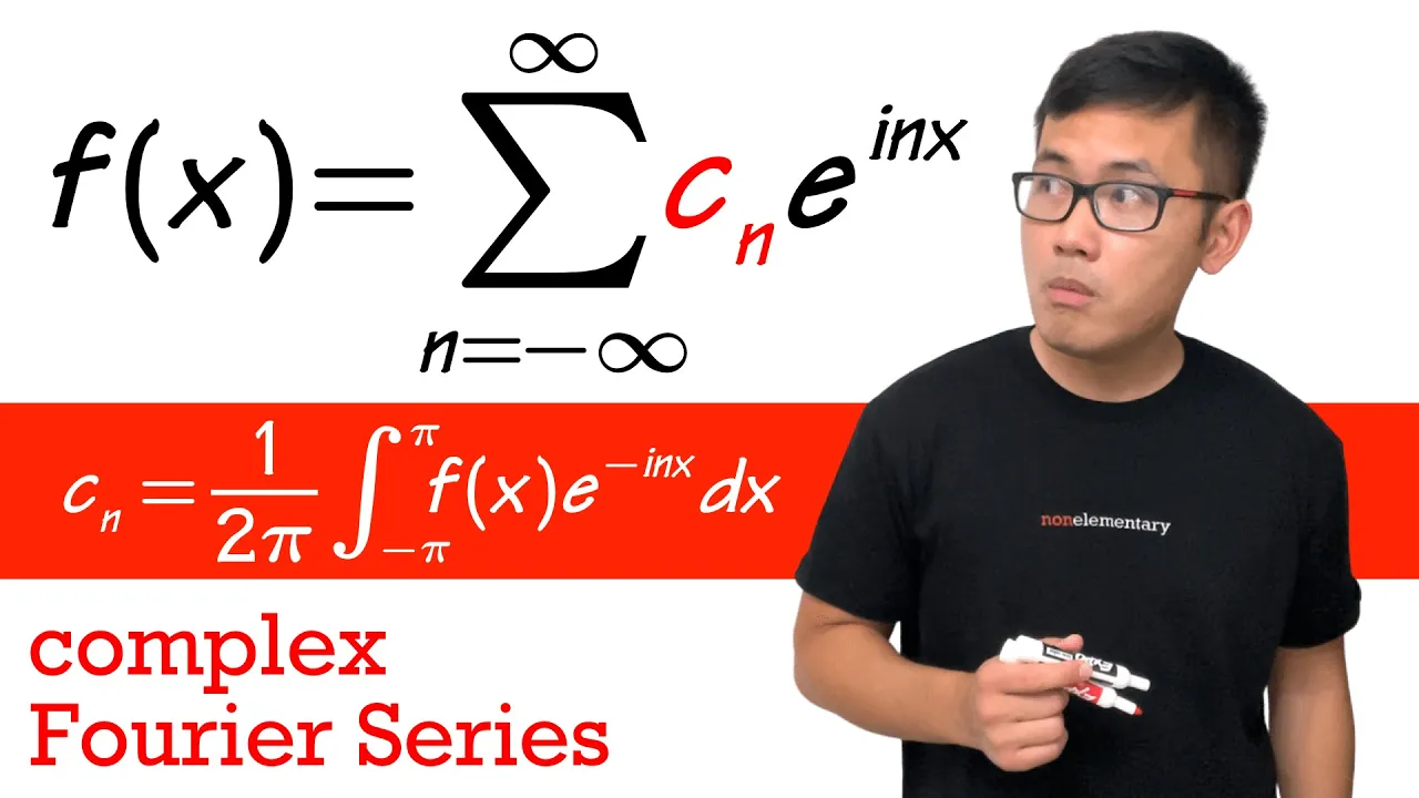
• Why this video: This video introduces the elegant complex exponential representation of the Fourier series ($f(x) = \sum C_ne^{inx}$). Moving to complex coefficients is critical for our transition to the continuous Fourier Transform in Module 3.
• Knowledge checkpoint:
  • Write the equation for the Complex Fourier Series and explain how the complex coefficients $C_n$ capture both amplitude and phase.
  • Calculate $C_n$ using the integral expression $C_n = \frac{1}{2\pi}\int_{-\pi}^{\pi} f(x)e^{-inx}dx$.
  • Understand how negative frequencies arise mathematically in the complex exponential domain.

Module 3: The Continuous Fourier Transform

This module bridges the gap between periodic and aperiodic signals. By mathematically taking the period of a periodic function to infinity ($T \to \infty$), you will watch discrete frequency spikes merge into a continuous frequency spectrum.

Review Note on Visual Gaps: This module contains excellent math lectures from Stanford. However, our video pool lacks the specific, famous 3Blue1Brown animation on the intuitive winding-machine view of the Fourier Transform. Independent Search Recommendation: We highly suggest searching YouTube for "3Blue1Brown But what is the Fourier Transform visual guide" to supplement this module's mathematical lectures with his classic visual animations.

Recommended Videos

Lecture 6 \| The Fourier Transforms and its Applications

@stanford47:52103938

Lecture 6 \| The Fourier Transforms and its Applications

The Fourier transform is derived as a limiting case of Fourier series by considering a non-periodic function that is zero outside some interval, periodizing it with increasingly larger periods T, computing the Fourier coefficients, and taking the limit as T approaches infinity. This process reveals that the discrete Fourier coefficients scale like 1/T and converge to a continuous function, leading to the Fourier transform definition: F(s) = ∫_{-∞}^∞ e^(-2πist) f(t) dt and the inverse transform f

@stanford · 47:52

• Why this video: This legendary Stanford lecture directly addresses our first major curriculum gap. It meticulously shows the step-by-step mathematical transition from the discrete Fourier Series to the continuous Fourier Transform by increasing the period $T \to \infty$.
• Knowledge checkpoint:
  • Mathematically demonstrate how increasing the period $T$ of a periodic function forces the discrete frequency steps ($\Delta f = 1/T$) to become infinitesimally small ($df$).
  • Formulate the continuous Fourier Transform analysis equation: $F(s) = \int_{-\infty}^{\infty} f(x)e^{-2\pi isx}dx$.
  • Explain how a continuous spectrum represents the frequency profile of non-repeating, transient signals.

Introduction to Fourier Transform

@nesoacademy08:19990002

Introduction to Fourier Transform

The Fourier Transform is a mathematical tool used for frequency analysis of signals, converting time-domain signals to frequency-domain representations. It exists for energy signals, power signals, and impulse-related signals, but not for signals that are neither energy nor power and not absolutely integrable. The Fourier Transform formula is X(jΩ) = ∫₋∞^∞ x(t)e^(-jΩt)dt, and the Inverse Fourier Transform is x(t) = (1/2π)∫₋∞^∞ X(jΩ)e^(jΩt)dΩ. The Fourier Transform can be derived from the Laplace

@nesoacademy · 08:19

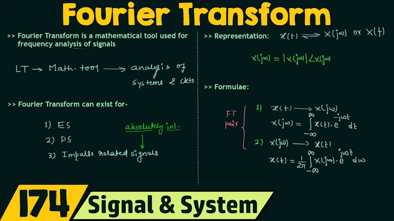
• Why this video: A clear, accessible overview of the physical and mathematical properties of the Fourier Transform. It is ideal for solidifying your structural understanding after tackling the heavy mathematical derivation from Stanford.
• Knowledge checkpoint:
  • Differentiate between energy signals and power signals as they relate to Fourier Transform convergence.
  • Contrast time-domain representation (amplitude over time) with frequency-domain representation (amplitude/phase over frequency).

Introduction to the Fourier Transform (Part 2)

@BrianBDouglas03:50531709

Introduction to the Fourier Transform (Part 2)

As the period T of a periodic function increases, the fundamental frequency decreases proportionally. Taking T → ∞ transforms periodic functions into aperiodic ones, yielding Fourier transform pairs from Fourier series. The orthogonality principle explains why multiplying signals at different frequencies yields zero: beat patterns create equal positive and negative areas that cancel out, meaning signals contain power only at their own fundamental frequencies.

@BrianBDouglas · 03:50

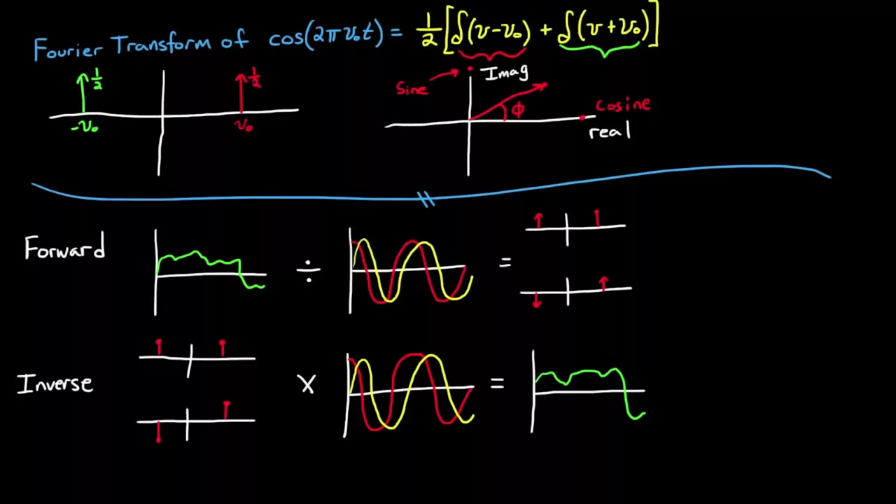
• Why this video: A short, highly-visual conceptual capture of the $T \to \infty$ limiting process. It provides excellent intuition on how discrete frequencies merge into a continuous domain.
• Knowledge checkpoint:
  • Describe the inverse relationship between the time-domain span of a window and its frequency-domain spread (fundamental scaling property).
  • Conceptualize how an impulse (delta) function in the time domain corresponds to a flat, infinite spectrum in the frequency domain.

Module 4: Sampling and the Discrete Fourier Transform (DFT)

To process signals on computers, we must convert continuous analog signals into finite, digital arrays. This module covers the mathematical framework of the sampling theorem, raw Discrete Fourier Transform (DFT) equations, and the highly optimized Fast Fourier Transform (FFT) algorithm.

Review Note on Raw DFT Gaps: Most educational resources rush straight to the Fast Fourier Transform (FFT) optimization. To ensure you master the raw DFT equation first (without the FFT speedup), we have selected targeted videos from VTU and SimonXu that explicitly walk through the raw DFT matrix and summation formulas.

Recommended Videos

Nyquist-Shannon; The Backbone of Digital Sound

@TechnologyConnections17:33582968

Nyquist-Shannon; The Backbone of Digital Sound

The Nyquist-Shannon sampling theorem states that a band-limited signal (one containing no frequencies above a certain limit) can be perfectly reconstructed from discrete samples taken at twice the rate of the highest frequency in the signal; this principle enables digital audio recording and playback, where signals are first band-limited using a low-pass filter (typically to 20 kHz for human hearing), then sampled at 40 kHz or higher, and finally reconstructed through a DAC with an identical low

@TechnologyConnections · 17:33

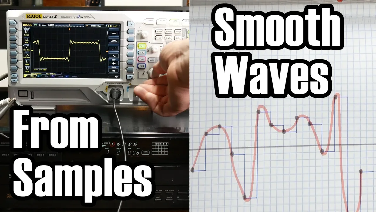
• Why this video: An exceptional, practical introduction to sampling theory. It demystifies why digital audio requires bandlimiting and why the sampling rate must exceed twice the highest frequency.
• Knowledge checkpoint:
  • State the Nyquist-Shannon Sampling Theorem and calculate the minimum sampling rate for a 20 kHz audio wave.
  • Explain the concept of "aliasing" and how it distorts signals when the Nyquist limit is violated.
  • Describe the function of an anti-aliasing filter in digital audio capture.

VTU DSP 18EC52 M1 L4 DFT and IDFT Equation

@canaraengineeringcollegema334004:023885

VTU DSP 18EC52 M1 L4 DFT and IDFT Equation

The DFT analysis equation transforms a time-domain signal into its frequency-domain representation. The equation is: X(k) = Σ (n=0 to N-1) x(n) × e^(-j2πkn/N), where x(n) is the input time-domain signal, X(k) is the output frequency-domain signal, N is the total number of samples, and k is the frequency index (bin number) varying from 0 to N-1. The equation is called the 'analysis equation' because it analyzes the time-domain signal to obtain frequency-domain samples. Both n and k are integers r

@canaraengineeringcollegema3340 · 04:02

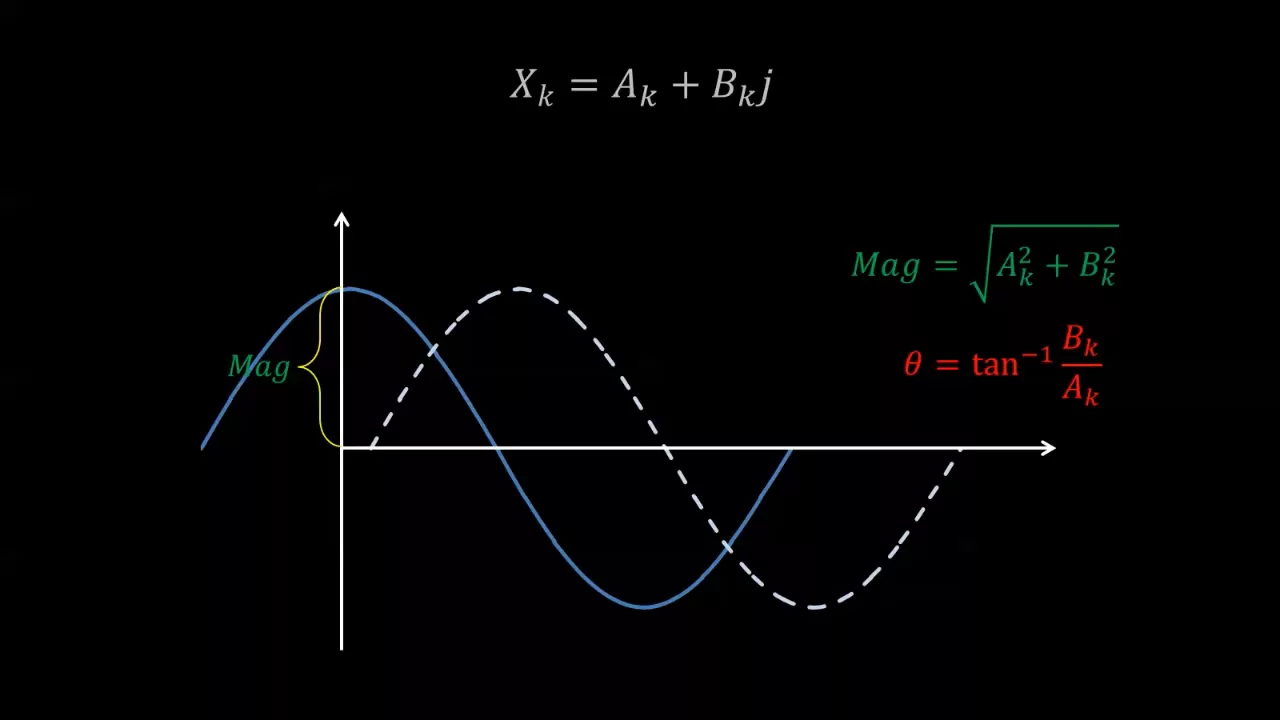
• Why this video: This video directly addresses our raw mathematical formula gap, detailing the structural mechanics of the DFT/IDFT analysis equations before any FFT optimizations are introduced.
• Knowledge checkpoint:
  • Write the mathematical analysis equation of the DFT: $X(k) = \sum_{n=0}^{N-1} x(n) e^{-j2\pi kn/N}$.
  • Define the variables $N$ (number of samples), $n$ (time index), and $k$ (frequency index).
  • Differentiate the Forward DFT equation from the Inverse DFT (IDFT) equation.

Discrete Fourier Transform - Simple Step by Step

@SimonXu10:34974509

Discrete Fourier Transform - Simple Step by Step

The Discrete Fourier Transform (DFT) converts a time-domain signal into its frequency components by multiplying the signal with complex exponentials (or equivalently sine and cosine waves) at different frequencies and summing the results; the resulting complex coefficients provide both the amplitude (magnitude) and phase shift of each frequency component, allowing us to analyze signals like white noise or pure tones by revealing which frequencies are present and their relative strengths.

@SimonXu · 10:34

• Why this video: This video offers an intuitive mathematical breakdown of the DFT equation, multiplying signal values with rotating complex vectors step-by-step to demonstrate how frequency bins are calculated.
• Knowledge checkpoint:
  • Compute a small $N=4$ DFT manually using the basic summation formula.
  • Understand why raw DFT computation possesses $O(N^2)$ computational complexity.
  • Explain how each index of the output array $X(k)$ represents the correlation of the input signal with a specific complex frequency.

The FFT Algorithm - Simple Step by Step

@SimonXu10:05255477

The FFT Algorithm - Simple Step by Step

The Fast Fourier Transform (FFT) is an efficient algorithm for computing the Discrete Fourier Transform (DFT) that reduces computational complexity from O(n²) to O(n log n) by exploiting the periodic nature of sinusoids through recursive decomposition into even and odd index summations, followed by combining intermediate results with exponential factors to compute all frequency bins.

@SimonXu · 10:05

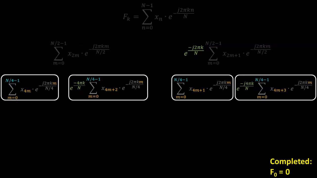
• Why this video: Learn how the Fast Fourier Transform (FFT) algorithm optimizes DFT calculations, reducing complexity from $O(N^2)$ to $O(N \log N)$ using divide-and-conquer principles.
• Knowledge checkpoint:
  • Explain the Cooley-Tukey algorithm's technique of splitting sequences into even and odd indices.
  • Define how the "twiddle factors" (complex roots of unity) enable computational reuse.
  • Recognize why the radix-2 FFT requires the input signal length $N$ to be a power of 2.

Module 5: Signal Processing Applications in the Real World

In this final module, you will discover practical applications of the Fourier Transform in digital systems, focusing on JPEG compression, the Discrete Cosine Transform (DCT), and real-time audio spectral visualization.

Recommended Videos

The Unreasonable Effectiveness of JPEG: A Signal Processing Approach

@Reducible34:481246043

The Unreasonable Effectiveness of JPEG: A Signal Processing Approach

JPEG achieves efficient image compression through a multi-stage mathematical process: it converts RGB images to YCbCr color space (separating brightness from color), applies chroma subsampling (exploiting human reduced sensitivity to color), performs the Discrete Cosine Transform (DCT) on 8x8 pixel blocks to convert spatial data to frequency coefficients, leverages the energy compaction property (concentrating most image energy in low-frequency coefficients), applies quantization (discarding hig

@Reducible · 34:48

• Why this video: This masterclass video breaks down JPEG's multi-stage mathematical pipeline, demonstrating how spatial images are represented in the frequency domain to exploit human visual limitations.
• Knowledge checkpoint:
  • Explain how JPEG uses the 2D Discrete Cosine Transform (DCT) on 8x8 pixel blocks to isolate high-frequency details.
  • Describe the difference between chroma subsampling, transformation, and quantization phases in lossy compression.
  • Identify how high-frequency coefficients are suppressed to zero during quantization to enable efficient compression.

JPEG DCT, Discrete Cosine Transform (JPEG Pt2)- Computerphile

@Computerphile15:11679075

JPEG DCT, Discrete Cosine Transform (JPEG Pt2)- Computerphile

JPEG compression works by converting an RGB image to YCbCr color space, then dividing it into 8x8 pixel blocks, applying the Discrete Cosine Transform (DCT) to represent each block as a sum of cosine waves with different frequencies, calculating coefficients for each wave, quantizing these coefficients to discard high-frequency information (which humans perceive less), and finally using Huffman encoding to compress the remaining data efficiently.

@Computerphile · 15:11

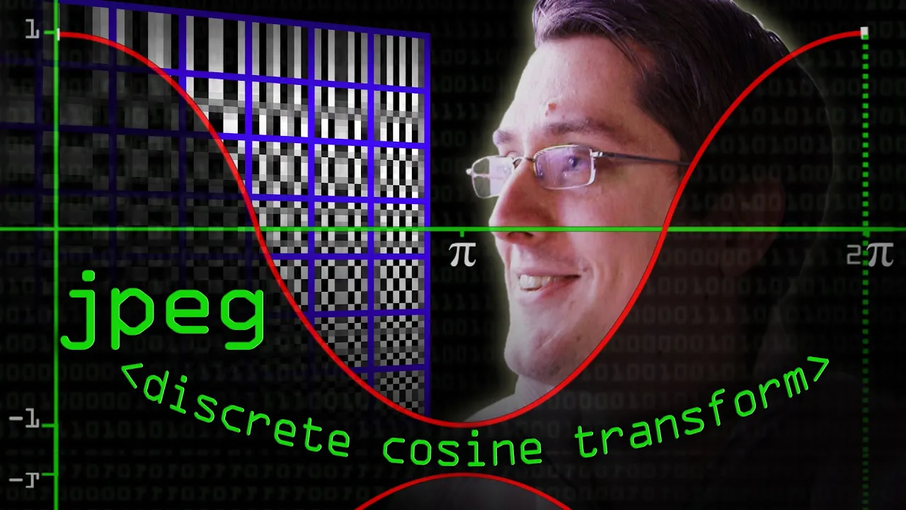
• Why this video: A fantastic, visual dive into how 2D DCT projects 8x8 blocks of pixels onto discrete 64 fixed basis cosine patterns, explaining why most high-frequency coefficients drop to zero.
• Knowledge checkpoint:
  • Define why a Discrete Cosine Transform (which uses only real-valued cosines) is preferred over a full complex Fourier transform for image block processing.
  • Conceptualize how quantization scales down high-frequency coefficients to enable efficient entropy coding.

17.11: Sound Visualization: Frequency Analysis with FFT - p5.js Sound Tutorial

@TheCodingTrain17:47287896

17.11: Sound Visualization: Frequency Analysis with FFT - p5.js Sound Tutorial

The p5.FFT object in p5.js performs Fast Fourier Transform (FFT) analysis on sound files, converting raw audio data into a spectrum array where each element represents the amplitude at a specific frequency level; this enables visualization of sound frequencies through graphic equalizers or circular displays, with the ability to adjust parameters like smoothing and bin count to control the resolution and appearance of the frequency analysis.

@TheCodingTrain · 17:47

• Why this video: To finalize the mathematical journey, this hands-on video demonstrates real-time FFT implementation in JavaScript (p5.js), mapping raw digital audio samples to a visual spectrum.
• Knowledge checkpoint:
  • Write logic to instantiate an FFT analyzer on a digital audio stream.
  • Explain how a frequency bin spectrum map translates sample values into visually reactive coordinates on a display.
  • Differentiate between sampling rate (determining frequency range) and FFT buffer size (determining frequency bin resolution).

Course Map

Key People Index

• Leonhard Euler (1707–1783): Developed Euler's formula ($e^{i\theta} = \cos\theta + i\sin\theta$) bridging trigonometry and complex analysis, providing the circular coordinate framework that forms the basis of modern signal processing.
• Jean-Baptiste Joseph Fourier (1768–1830): Pioneered the mathematical theorem that periodic functions can be represented as an infinite sum of trigonometric series, laying the foundation for frequency-domain analysis.
• Harry Nyquist (1889–1976) & Claude Shannon (1916–2001): Formulated and proved the Nyquist-Shannon Sampling Theorem, establishing the absolute mathematical rules governing the transition between analog waveforms and digital data.
• Carl Friedrich Gauss (1777–1855) / James Cooley (1926–2016) & John Tukey (1915–2000): Gauss originally discovered the Cooley-Tukey FFT algorithm structure in 1805 (unpublished), which was later re-discovered and popularized by Cooley and Tukey in 1965, optimizing DFT computation and making real-time digital computing possible.

Final Self-Assessment

Complete this comprehensive self-assessment to verify your mastery of the Fourier Transform curriculum.

• Can you visually construct Euler's formula on the complex plane and use it to represent rotating vectors (phasors)?
• Can you define mathematical orthogonality and explain how it allows us to project functions to extract specific Fourier coefficients?
• Do you understand the physical and mathematical limit where the periodic period $T \to \infty$, morphing the Fourier Series into the continuous Fourier Transform?
• Can you write out the analysis equations for both the Continuous Fourier Transform and the Discrete Fourier Transform (DFT)?
• Do you understand how sampling rate affects signal reconstruction and how to calculate the Nyquist rate for a given bandwidth?
• Can you explain the structural divide-and-conquer strategy behind the Fast Fourier Transform (FFT)?
• Can you explain the role of the 2D Discrete Cosine Transform (DCT) in lossy JPEG compression?
• Can you describe how an FFT object converts raw temporal audio amplitude data into discrete frequency bin arrays for spectral analysis?