Numerical Analysis: Roots, Splines & Errors

Learning Goal: Numerical Analysis and Approximation Algorithms: Constructing interpolating polynomials, splines, root-finding methods, and error propagation analysis.

This curriculum provides a structured, video-based learning path designed to transition you from an understanding of binary representation errors to master-level formulation of interpolation, splines, root-finding, and integration approximations.

• Prerequisites: Multivariable Calculus, Taylor Series expansions, and basic linear algebra (matrix systems).
• Estimated Total Study Time: 18 Hours.

Module 1: Computer Arithmetic and Error Analysis

This module introduces how computers store real numbers, the mathematical limits of floating-point arithmetic, and how small initial round-off and truncation errors propagate through long sequences of computations.

Floating Point Representation and Rounding Error

@countingonjustice03:3595,983

Floating Point Representation and Rounding Error

Machine epsilon (ε) measures the gap between 1 and the next representable number in double precision: ε = 2^(-52) ≈ 10^(-16). Absolute error is the difference between actual and stored values. Relative rounding error = absolute error / true number. For repeating decimals like 9.4 (binary 1001.0110...), truncation creates errors that accumulate. The relative rounding error is always ≤ ε/2, providing a theoretical bound on computational errors.

@countingonjustice · 03:35

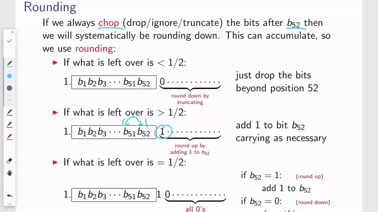
• Why this video: This video offers an intuitive, bite-sized breakdown of how floating-point numbers represent approximations of real numbers. It defines absolute error vs. relative error and introduces machine epsilon ($\varepsilon$) under standard double precision ($2^{-52} \approx 10^{-16}$).

1.1 Floating Point Data (Numerical Analysis)

@drewmacha10:25133

1.1 Floating Point Data (Numerical Analysis)

This section introduces machine epsilon as a measure of relative roundoff error in floating point computations. Machine epsilon equals half the gap between 1 and the next representable number larger than 1, calculated as 2^(1 - n) for n mantissa bits. For 10 mantissa bits, machine epsilon = 2^(-9) ≈ 0.001953125. The instructor explains that absolute error |x - x̂| ≤ machine epsilon × |x| for any real number x and its closest approximation x̂. Relative error is preferred over absolute error becau

@drewmacha · 10:25

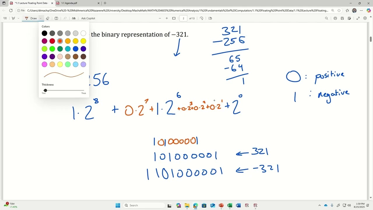
• Why this video: Addressing the feedback for a rigorous explanation of machine epsilon, this academic tutorial explains how to measure relative round-off errors. It derives the exact mathematical relationship between machine epsilon and the representation gap on the real line.

P. Habala, DEN-01b: Numerical analysis – Errors and their propagation in calculations

@CVUTFEL01:19:39367

P. Habala, DEN-01b: Numerical analysis – Errors and their propagation in calculations

In numerical analysis, errors propagate differently through arithmetic operations: addition/subtraction preserve relative error quality, while multiplication/division approximately double the relative error per operation, and subtraction of nearly equal numbers can cause catastrophic cancellation where small input errors produce large output errors, making numerical stability crucial for reliable computations.

@CVUTFEL · 01:19:39

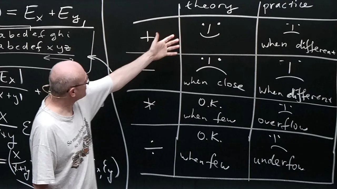
• Why this video: This highly rigorous lecture covers how errors propagate through foundational mathematical operations. It demonstrates why addition and subtraction can preserve or worsen relative error bounds, while multiplication and division amplify relative uncertainties.

Knowledge Checkpoint

• Define machine epsilon ($\varepsilon$) mathematically and explain how it limits computer representation of decimals.
• Calculate the absolute and relative error bounds of a floating-point calculation.
• Identify subtraction cancellation and explain why subtracting two nearly identical float values leads to severe loss of significance.

Module 2: Root-Finding Methods

This module shifts focus to solving $f(x) = 0$ for non-linear equations. It reviews the visual, geometric, and algorithmic construction of Bisection, Secant, and Newton-Raphson methods, comparing their computational cost and rate of convergence.

Engineering Mathematics || GATE & ESE || Numerical Methods || Lec-02

@engineershub895403:1110,188

Engineering Mathematics || GATE & ESE || Numerical Methods || Lec-02

The bisection method proceeds as follows: (1) Start with interval [a, b] where f(a) and f(b) have opposite signs; (2) Compute midpoint c = (a+b)/2; (3) Evaluate f(c); (4) If f(c) = 0, c is the root; (5) If f(a) and f(c) have opposite signs, set b = c; else set a = c; (6) Repeat until desired accuracy is achieved. For the equation x⁴ - 5x³ - 2x² - 4x - 1 = 0 in [1, 9], the root was found at x = 2 after 3 iterations.

@engineershub8954 · 03:11

• Why this video: Directly filling the gap identified in the review feedback, this video outlines a step-by-step walkthrough of the Bisection Method. It shows how the algorithm uses continuous interval boundaries to narrow down the root range systematically.

Root finding: The Newton method

@CVUTFEL08:11198

Root finding: The Newton method

Convergence rate quantifies how quickly sequences approach limits. Linear convergence (Q=1) adds constant digits per iteration; superlinear convergence improves faster; quadratic convergence (Q=2) doubles correct digits per step. The general definition compares successive errors: |x_{k+1}-r| ≤ C|x_k-r|^Q. Higher exponents yield dramatically faster convergence, transforming practical computation times.

@CVUTFEL · 08:11

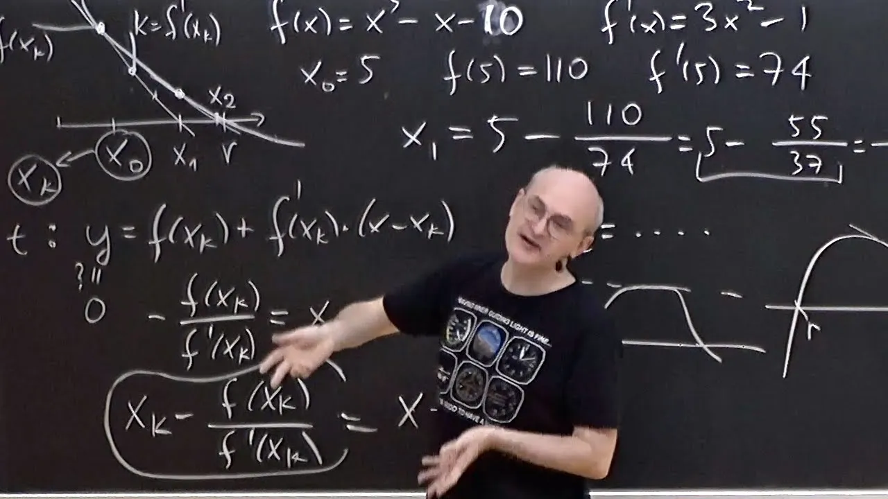
• Why this video: This video bridges the gap regarding convergence rates. It compares linear convergence (Q=1, constant digits added per step) and quadratic convergence (Q=2, doubling the correct digits per iteration), explaining why the Newton-Raphson method achieves quadratic speed under optimal conditions.

Root finding: The secant method

@CVUTFEL05:13118

Root finding: The secant method

Practical method comparison should consider computational cost per iteration rather than pure mathematical order. The secant method requires only one function evaluation per iteration (reusing previous values), while Newton needs two. Converting Newton's order-2 performance to single-evaluation basis yields effective order ~1.414, making secant's practical rate (~1.6) superior. When measured by actual time spent computing, two secant iterations achieve error reduction ~e^3.2 versus Newton's e² p

@CVUTFEL · 05:13

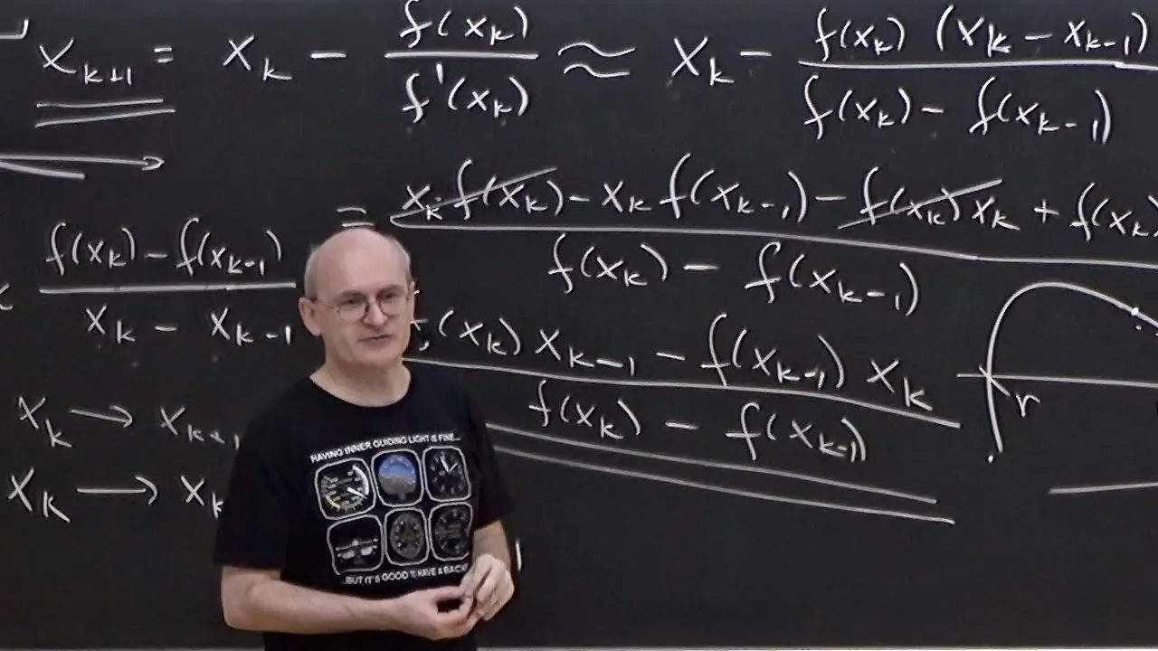
• Why this video: The Secant Method is introduced as a derivative-free alternative to Newton's method. This presentation analyzes the practical comparison between these two methods, highlighting computational costs per iteration.

Knowledge Checkpoint

• Determine when a root-finding algorithm will converge and state the convergence criteria.
• Contrast the convergence rates of the Bisection (linear), Secant (superlinear, $\approx 1.618$), and Newton-Raphson (quadratic) methods.
• Perform a manual 3-step iteration of the Newton-Raphson method for a transcendental equation.

Module 3: Polynomial Interpolation & Runge's Phenomenon

This module covers polynomial interpolation, exploring how to build unique, lower-degree polynomials that pass through discrete data nodes. It introduces Lagrange and Newton formulations, then investigates Runge's phenomenon—the wild oscillations that happen at interval edges when using high-degree polynomials.

Lagrange Interpolating Polynomial - Easy Method

@AFMathandEngineering08:10330,202

Lagrange Interpolating Polynomial - Easy Method

The Lagrange interpolating polynomial is a method for estimating function values at intermediate points by constructing a polynomial that passes through given data points; the process involves creating terms for each data point where each term equals the y-value multiplied by a fraction: the numerator contains (x minus all other x-values) and the denominator contains (the current x-value minus all other x-values), with all terms summed together before evaluating at the desired x-value.

@AFMathandEngineering · 08:10

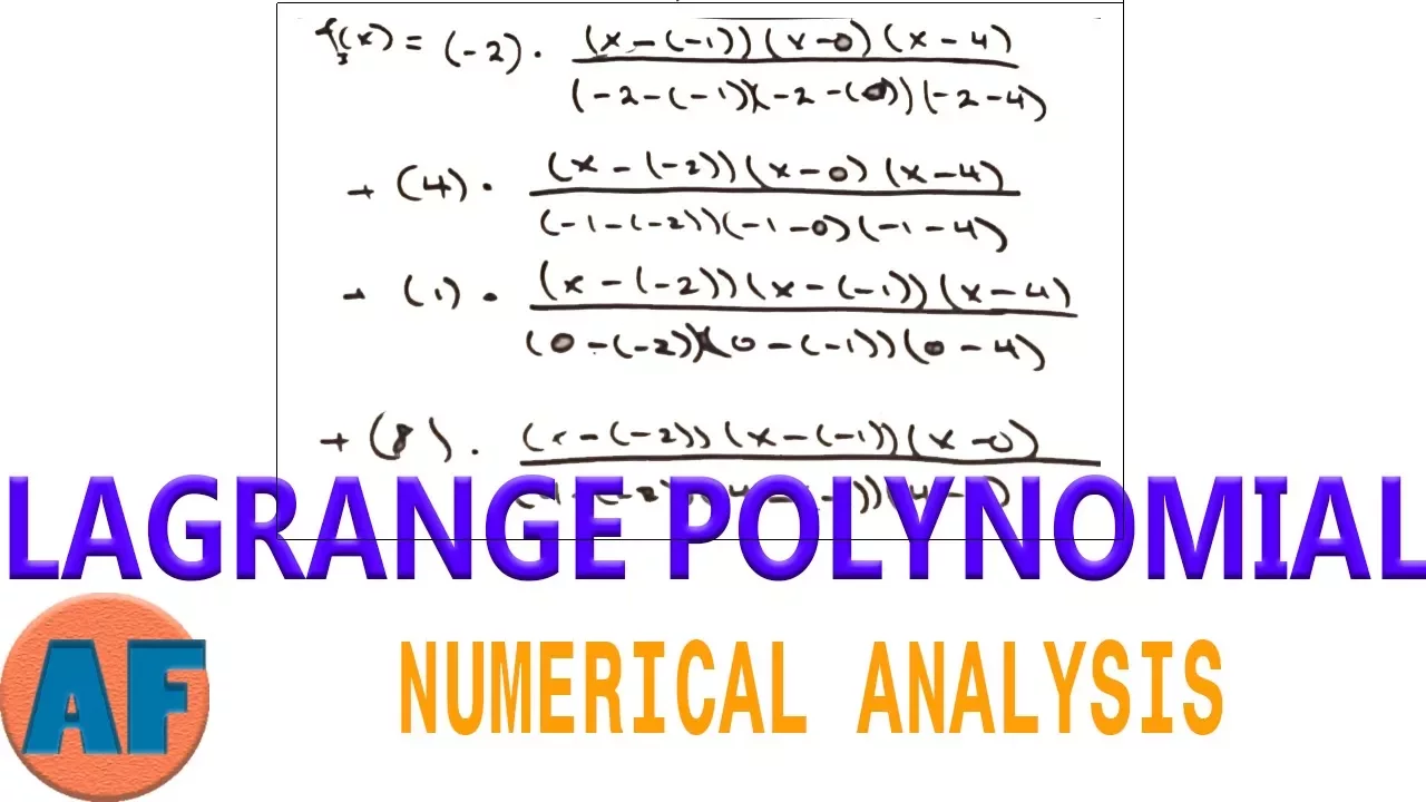
• Why this video: This practical guide walks through constructing Lagrange basis polynomials ($L_i(x)$) from scratch. It demonstrates the mechanics of fitting a single polynomial curve through target coordinates.

NEWTON DIVIDED DIFFERENCE FORMULA - secret TIPS & TRICKS | NUMERICAL METHOD | TUTORIAL - 3

@IclassesForYou01:10191,245

NEWTON DIVIDED DIFFERENCE FORMULA - secret TIPS & TRICKS | NUMERICAL METHOD | TUTORIAL - 3

The formula is: y = f(x₀) + (x-x₀) × f[x₀,x₁] + (x-x₀)(x-x₁) × f[x₀,x₁,x₂] + (x-x₀)(x-x₁)(x-x₂) × f[x₀,x₁,x₂,x₃] + ... + (x-x₀)(x-x₁)...(x-xₙ₋₁) × f[x₀,x₁,...,xₙ]. For example, with x₀=2, x₁=3, x₂=6, x₃=7, x₄=9, and f(x₀)=15, the formula becomes: y = 15 + (x-2)×24 + (x-2)(x-3)×11 + (x-2)(x-3)(x-6)×1 + (x-2)(x-3)(x-6)(x-7)×0.

@IclassesForYou · 01:10

• Why this video: Building on Lagrange's formulation, this lesson covers Newton's divided-difference method. It explains how to build divided-difference tables recursively, presenting a more computationally efficient format for adding new nodes.

Interpolation - Cubic Splines - Basics

@the-Math-guy03:0988,559

Interpolation - Cubic Splines - Basics

High-order polynomial interpolation suffers from oscillatory behavior known as Runge's phenomenon, where increasing polynomial degree leads to more turning points and severe oscillations, particularly at interval endpoints. Fitting a 14th-16th order polynomial to approximate functions like 1/(1+x²) produces significant oscillations despite reasonable central approximations. This motivates spline interpolation, which divides data into smaller segments and fits lower-degree polynomials between con

@the-Math-guy · 03:09

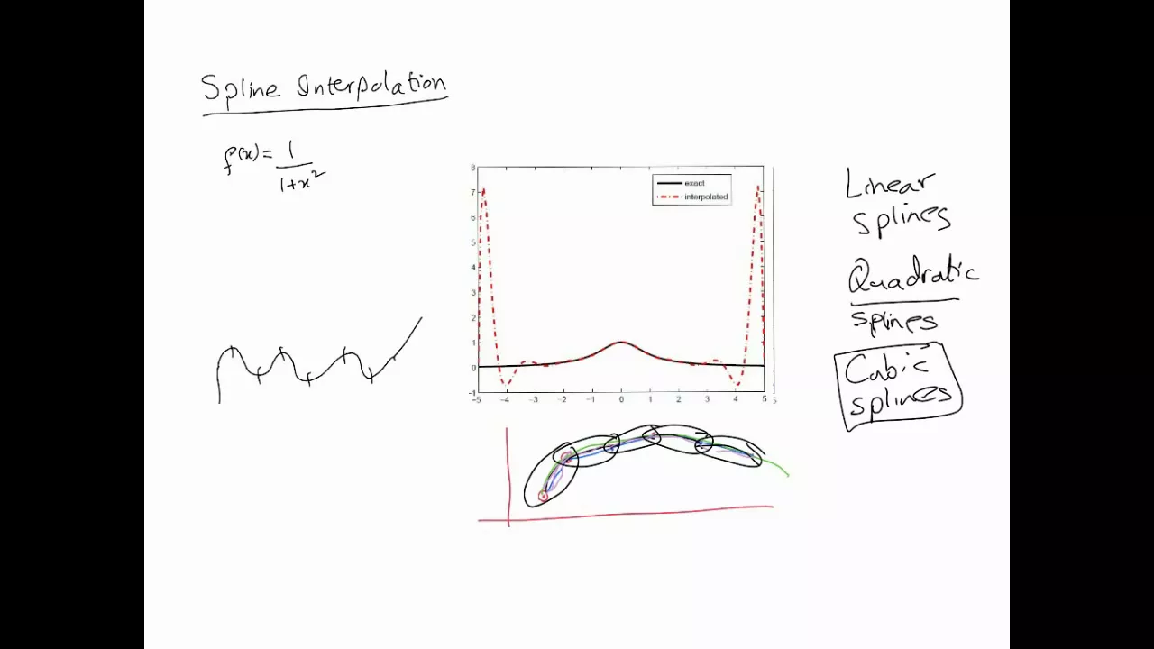
• Why this video: To address the gap concerning Runge's phenomenon, this tutorial visualizes how increasing the degree of an interpolating polynomial over equidistant points causes wild oscillations near the interval boundaries. This highlights the limits of global polynomial models.

Knowledge Checkpoint

• Formulate a Lagrange polynomial $P_n(x)$ given $n+1$ distinct points.
• Build a complete divided-difference table and write out the corresponding interpolating polynomial.
• Define Runge's phenomenon and explain why equidistant node distribution makes high-degree global polynomial interpolation unstable.

Module 4: Spline Interpolation & Piecewise Approximation

This module introduces spline interpolation, which avoids Runge's phenomenon by using low-degree piecewise polynomials instead of a single high-degree polynomial. You will learn to construct piecewise linear and cubic splines that maintain smoothness across boundaries.

ch3 5: Natural Cubic Splines; Derivation of Algorithm. Wen Shen

@wenshenpsu14:4723,146

ch3 5: Natural Cubic Splines; Derivation of Algorithm. Wen Shen

Natural cubic splines are piecewise cubic polynomials that interpolate data points with continuous first and second derivatives, where the second derivatives at the endpoints are zero; the algorithm involves defining unknown second derivative values Z_i at interior knots, expressing the spline in Lagrange form, integrating twice to obtain the cubic polynomial, applying interpolation conditions to derive relationships between coefficients, enforcing continuity of the first derivative to form a tr

@wenshenpsu · 14:47

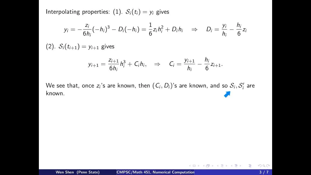
• Why this video: This video provides a step-by-step mathematical derivation of natural cubic splines. It explains how to enforce continuous first ($S'$) and second ($S''$) derivatives at internal boundaries, and how setting second derivatives to zero at the endpoints leads to a solvable tri-diagonal matrix system.

Interpolation - Cubic Splines - example

@the-Math-guy13:20258,085

Interpolation - Cubic Splines - example

This comprehensive process covers constructing a natural cubic spline that passes through given data points. The method involves: (1) dividing the interval into subintervals with corresponding cubic polynomials; (2) applying point matching conditions to ensure the spline passes through each data point; (3) enforcing continuity of first and second derivatives at interior points; (4) applying natural boundary conditions (zero second derivatives at endpoints); (5) forming a system of linear equatio

@the-Math-guy · 13:20

• Why this video: This tutorial walks through a complete numerical example of building a cubic spline. It shows how to translate interpolation coordinates and continuity requirements into a system of linear equations, and how to solve for the spline's coefficients.

Knowledge Checkpoint

• Explain why cubic splines are preferred over linear and quadratic splines for modeling physical processes.
• Write down the boundary and continuity equations that define a natural cubic spline at an interior node $x_i$.
• Set up the tri-diagonal linear system of equations needed to solve for the spline parameters of a four-point data set.

Module 5: Numerical Integration & Error Bounds

This module covers approximating definite integrals using Newton-Cotes rules. It introduces the composite Trapezoidal and Simpson's rules, while examining how discretization sizes affect approximation errors.

The Trapezoid Rule for Approximating Integrals

@patrickjmt06:42661,160

The Trapezoid Rule for Approximating Integrals

The trapezoidal rule approximates definite integrals by dividing the area under a curve into trapezoids. The formula is: (Δx/2) × [f(x₀) + 2f(x₁) + 2f(x₂) + ... + 2f(xₙ₋₁) + f(xₙ)], where Δx = (B - A)/n. First, calculate Δx by dividing the interval length by the number of trapezoids. Then evaluate the function at each endpoint and midpoint, multiplying all intermediate values by 2. Finally, multiply the sum by Δx/2. For f(x) = 1 + x² from 1 to 5 with 4 trapezoids, Δx = 1, and the approximation y

@patrickjmt · 06:42

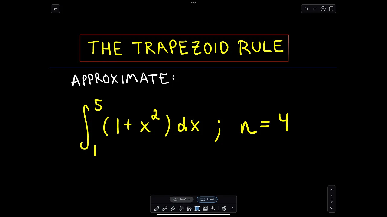
• Why this video: This video provides an easy-to-follow, visual introduction to the composite Trapezoidal Rule. It details how the formula approximates the area under a curve using trapezoids and walks through a manual calculation step-by-step.

Simpson's Rule & Numerical Integration

@TheOrganicChemistryTutor12:11812,914

Simpson's Rule & Numerical Integration

Simpson's Rule is a numerical integration technique that approximates the definite integral of a function by dividing the interval [a, b] into n subintervals (where n is even), calculating the width Δx = (b-a)/n, and applying the formula Sₙ = (Δx/3)[f(x₀) + 4f(x₁) + 2f(x₂) + 4f(x₃) + ... + 4f(xₙ₋₁) + f(xₙ)], where coefficients alternate between 4 and 2 for interior points starting with 4 for x₁, making it particularly effective for estimating integrals when only discrete data points are availabl

@TheOrganicChemistryTutor · 12:11

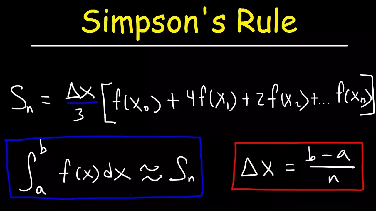
• Why this video: This tutorial covers Simpson's 1/3 Rule, which fits parabolic arcs to three points at a time. It highlights the requirement for an even number of subintervals ($n$) and demonstrates the 1-4-2-4-...-1 weighting pattern.

Error in quadrature Formulae. L-3 by Dr Rekha Srivastava L. U.

@lucknowuniversitymathemati68714:084,170

Error in quadrature Formulae. L-3 by Dr Rekha Srivastava L. U.

This comprehensive lesson covers the error analysis of numerical integration methods. The general error formula is E = ∫f(x)dx - Q[f]. For the trapezoidal rule, Taylor series expansion yields principal error -h³/12 f''(x₀), with total error E < (b-a)h²/12 × M (order h²). For Simpson's one-third rule, the principal error is -2h⁴/3 f'''(x₀), with total error E < (b-a)h³/3 × M (order h⁴). The derivation involves expanding f(x) about x₀, integrating, and comparing with the numerical approximation. H

@lucknowuniversitymathemati687 · 14:08

• Why this video: This lecture analyzes the mathematical error bounds of these integration rules. It uses Taylor series expansions to derive the principal error terms and evaluate the truncation errors of both the Trapezoidal and Simpson's formulas.

Knowledge Checkpoint

• State the degree of precision for both the Trapezoidal Rule (degree 1) and Simpson's Rule (degree 3).
• Approximate a definite integral using composite Simpson's 1/3 Rule given a step-size $h$.
• Determine the maximum step size $h$ required to approximate an integral within a specified error tolerance using the Trapezoidal Rule error bound formula.

Course Map

This map outlines the recommended progression and dependencies for this curriculum.

Key People Index

• Carl Runge (1856–1927): German mathematician who discovered that high-degree polynomial interpolation on equidistant points leads to severe oscillation errors near the boundaries.
• Isaac Newton (1643–1727): Developed the Newton-Raphson root-finding algorithm, Newton divided-difference interpolation, and Newton-Cotes integration formulas.
• Joseph-Louis Lagrange (1736–1813): Formulated the Lagrange interpolation technique using Lagrange basis polynomials.
• Thomas Simpson (1710–1761): English mathematician who popularized Simpson's rule, approximating definite integrals using parabolic arcs.

Final Self-Assessment

Test your understanding of the curriculum with these final objectives:

• Calculate the absolute and relative representation error of a real number in single or double precision binary float representation.
• Find the root of $f(x) = 0$ using the Bisection method to within a specified tolerance $10^{-k}$.
• Compute the derivative of $f(x)$ to perform the Newton-Raphson method and state what conditions would cause the method to fail (e.g., $f'(x) = 0$ or cycling).
• Construct the Newton divided-difference table for five data points and evaluate the resulting interpolating polynomial at an arbitrary point.
• Graphically sketch Runge's phenomenon and explain how Chebyshev node spacing can mitigate it.
• Write down the complete system of boundary and continuity equations that define a cubic spline.
• Prove why a "natural" spline is called "natural" by showing its boundary constraints at the endpoints.
• Approximate a definite integral using composite Simpson’s 1/3 rule and compute its error bound using the fourth derivative of the function.