Orbital Mechanics: Kepler, Hohmann & Assists

Learning Goal: Mastering the principles of orbital mechanics and interplanetary trajectory design, including Keplerian elements, Hohmann transfer orbits, gravity assists, and the utilization of Lagrangian points.

• Prerequisites: Vector calculus, introductory classical mechanics (Newton's laws, rotational dynamics), and basic python/programming exposure (highly recommended for numerical implementations).
• Estimated Total Study Time: 28 hours

Module 1: Foundations of Astrodynamics

This module establishes the core mathematical and physical framework of orbital mechanics. You will move from the conceptual elegance of Kepler’s three laws of planetary motion to the rigorous mathematical derivations of Newtonian gravitation, centripetal forces, and energy conservation. This module addresses the feedback of missing mathematical rigor by providing full-length academic lectures alongside visual explainers.

Recommended Videos

Astrodynamics UF Lecture4 2017 (Newton's Gravitation Law)

@riccardobevilacqua984933:08605

Astrodynamics UF Lecture4 2017 (Newton's Gravitation Law)

Newton's law of gravitation states that two point masses attract each other with force F = G M1 M2 / R², where G ≈ 6.674 × 10⁻¹¹ N·m²/kg². Gravitational acceleration is a = G M1 / R², depending only on the attracting body's mass and distance. The law applies to spherical bodies with uniform mass distribution, allowing planets to be treated as point masses. The vector form is F12 = G M1 M2 / R² * û12. Gravitational forces are conservative, allowing potential energy V = -G M1 M2 / R, with force ob

@riccardobevilacqua9849 · 33:08

Why this video is valuable: This university-level lecture provides the mathematical foundation of Newtonian gravity required for professional astrodynamics. It rigorously derives the gravitational acceleration vector ($a = - \frac{G M}{R^2} \hat{u}_r$) and explores the dependency of gravitational attraction on point masses. This academic deep-dive directly addresses the review feedback by ensuring you master the calculus-based derivations of orbital motion, rather than relying solely on conceptual hand-waving.

HOW IT WORKS: Orbital Mechanics

@TheDocumenteriesTube34:24515,727

HOW IT WORKS: Orbital Mechanics

Orbital mechanics is the study of how celestial bodies move under gravitational forces, governed by Kepler's three laws of planetary motion (elliptical orbits, equal area sweep, and period-distance relationship) and Newton's universal gravitation and three laws of motion, which together explain why satellites stay in orbit and how spacecraft can be launched, maneuvered, and controlled in space.

@TheDocumenteriesTube · 34:24

Why this video is valuable: This highly detailed and comprehensive documentary systematically bridges the gap between historical Keplerian observations and modern orbital operations. It explains how Kepler's three laws (elliptical paths, equal area sweep over equal time, and the square of the orbital period relation to the cube of the semi-major axis) manifest in real-world systems. It provides an excellent transition from historical physics to applied astrodynamics.

Gravity for astronauts in orbit | Centripetal force and gravitation | Physics | Khan Academy

@khanacademy03:49286,638

Gravity for astronauts in orbit | Centripetal force and gravitation | Physics | Khan Academy

Newton's law of universal gravitation states that gravitational force equals G(m₁m₂)/r², where r is the distance between centers. For objects near Earth's surface or in low Earth orbit, r doesn't change dramatically in percentage terms, meaning gravitational force remains substantial. Astronauts aren't in zero gravity but are in continuous free fall toward Earth. They move horizontally fast enough that they 'miss' Earth as they fall, creating an orbit. The gravitational pull constantly curves th

@khanacademy · 03:49

Why this video is valuable: This video focuses on the fundamental balance of forces in low Earth orbit. It mathematically unpacks how centripetal acceleration ($a_c = \frac{v^2}{r}$) must equal the gravitational acceleration to maintain a circular orbit. It explains why astronauts experience weightlessness not due to a lack of gravity, but because they are in a perpetual state of free fall.

Knowledge Checkpoint

• Derive the acceleration equation of a satellite under a central gravitational field using Newton's Law of Gravitation.
• State Kepler’s three laws of planetary motion and explain how the conservation of angular momentum supports the Second Law (equal areas in equal time).
• Calculate the velocity required to maintain a circular orbit at a given altitude ($r$) using the relation $v = \sqrt{\frac{\mu}{r}}$, where $\mu = GM$.
• Explain the relationship between total orbital energy ($E = K + U$) and orbit geometry (elliptical, parabolic, hyperbolic).

Module 2: Keplerian Orbits and Orbital Elements

To define a spacecraft’s state vector in three-dimensional space, we utilize the six Keplerian orbital elements. This module systematically details these six parameters and covers how they uniquely map to position and velocity vectors ($\vec{r}, \vec{v}$).

Note: Real-world coordinate system transformations (such as converting from the Geocentric Equatorial frame to the Perifocal frame) are mathematically dense; you are strongly encouraged to complement these videos by practicing matrix rotations using Direction Cosine Matrices (DCM).

Recommended Videos

Part 1: The Orbital Elements (ORBITER Tutorial Series for Beginners)

@TexFilms11:4767,496

Part 1: The Orbital Elements (ORBITER Tutorial Series for Beginners)

The six orbital elements—semi-major axis (defining orbit size and period), eccentricity (defining orbit shape from 0 for circular to 1+ for escape trajectories), inclination (angle between orbital plane and reference plane), longitude of ascending node (angle from reference direction to ascending node), argument of periapsis (angle from ascending node to periapsis), and time of periapsis passage (locating position in orbit)—completely specify an unperturbed orbit in space, with prograde burns in

@TexFilms · 11:47

Why this video is valuable: This tutorial offers an intuitive, visual walkthrough of how the six classical orbital elements define an orbit's size, shape, and spatial orientation. It provides a visual frame of reference that makes abstract parameters—such as the Right Ascension of the Ascending Node (RAAN) and Argument of Periapsis—instantly clear.

Keplerian Orbital Elements Introduction | Fundamentals of Orbital Mechanics 5

@alfonsogonzalez-astrodynam220703:4816,829

Keplerian Orbital Elements Introduction | Fundamentals of Orbital Mechanics 5

This section covers the foundational concepts of orbital mechanics including periapsis (closest point to Earth), apoapsis (farthest point), and the apse line connecting them. The semi-major axis is calculated as the average of apoapsis and periapsis and determines orbital period. Eccentricity measures orbital circularity, ranging from 0 (circular) to 1 (highly elliptical). Orbital inclination describes the tilt of the orbital plane relative to Earth's equatorial plane, with values between 0-90°

@alfonsogonzalez-astrodynam2207 · 03:48

Why this video is valuable: Alfonso Gonzalez’s orbital mechanics series is renowned for its mathematical precision and clear code integrations. This video introduces the foundational geometry of Keplerian elements, covering the periapsis, apoapsis, and the apse line. It lays the groundwork for representing spacecraft state vectors and transitions from pure geometric visualization to algorithmic design.

Classical/Keplerian Orbital Elements

@SpaceflightScience04:15142,413

Classical/Keplerian Orbital Elements

This section introduces the foundational principles of orbital mechanics. Kepler's first law states that all orbits are ellipses with the central body at one focal point. An ellipse has a major axis (long axis) and minor axis (short axis), with the closest point called periapsis and the furthest point called apoapsis. The size of an orbit is determined by the semi-major axis (half the major axis), denoted by 'a'. The shape is determined by eccentricity (denoted by 'e'), which measures how elonga

@SpaceflightScience · 04:15

Why this video is valuable: This segment isolates the specific geometry of orbits, breaking down the semi-major axis ($a$), eccentricity ($e$), and inclination ($i$). It serves as an excellent resource for establishing the geometric limits of Kepler's First Law, showcasing how a circular orbit is simply a specialized boundary case of a generalized ellipse where $e=0$.

Knowledge Checkpoint

• Define the six classical Keplerian orbital elements ($a$, $e$, $i$, $\Omega$, $\omega$, $\nu$) and explain the physical meaning of each.
• Identify which orbital elements define the size and shape of the orbit, which define its spatial orientation, and which defines the spacecraft's current position.
• Differentiate between the perifocal coordinate frame ($PQW$) and the geocentric equatorial coordinate frame ($IJK$).
• Explain the geometric relationship between the semi-major axis ($a$), periapsis radius ($r_p$), apoapsis radius ($r_a$), and eccentricity ($e$) using the equations $r_p = a(1-e)$ and $r_a = a(1+e)$.

Module 3: Orbital Maneuvers and Hohmann Transfers

To navigate space, spacecraft must alter their orbital parameters by expending propellant. This module moves beyond basic pop-science overviews to focus on the calculations of delta-v ($\Delta v$) for coplanar orbital transfers (Hohmann and bi-elliptic transfers) and orbital plane changes.

Recommended Videos

5 - 4 - Impulsive Maneuvers and Co-Planar Orbital Transfers

@dsavransky03:23730

5 - 4 - Impulsive Maneuvers and Co-Planar Orbital Transfers

Bi-elliptic transfers use three burns instead of two, potentially offering greater efficiency than Hohmann transfers for specific orbit ratios. The maneuver involves: (1) a tangential burn at initial orbit to enter first transfer ellipse, (2) a second burn at intermediate point (radius r_t) to enter second transfer ellipse, (3) a third burn at final orbit to match velocity. This approach exploits gravitational potential energy differences at various altitudes. The efficiency threshold occurs at

@dsavransky · 03:23

Why this video is valuable: This lecture focuses on the math of impulsive maneuvers. It directly addresses a major gap highlighted in the review feedback: the mathematical explanation of bi-elliptic transfers. It covers how a three-burn bi-elliptic transfer uses an intermediate high apoapsis to change orbits and explains why, for large ratios of final to initial semi-major axes ($R > 11.94$), a bi-elliptic transfer is actually more fuel-efficient than a standard two-burn Hohmann transfer.

Interplanetary Hohmann Transfers: Delta-V and Time of Flight Calculations

@alfonsogonzalez-astrodynam220703:0711,067

Interplanetary Hohmann Transfers: Delta-V and Time of Flight Calculations

Hohmann transfer analysis involves calculating two critical delta-v burns: the first equals transfer orbit velocity minus departure planet's circular velocity (Δv₁ = v_transfer_departure - v_planet_departure), while the second equals arrival planet's circular velocity minus transfer orbit velocity at arrival (Δv₂ = v_planet_arrival - v_transfer_arrival). The time of flight equals half the transfer orbit period, calculated as T = π × √(a³/μ). For Earth-to-Mars transfers, this yields approximately

@alfonsogonzalez-astrodynam2207 · 03:07

Why this video is valuable: This tutorial outlines the step-by-step mathematical calculations needed to design a transfer trajectory from a departure planet's circular orbit to a target planet. It details how to calculate the initial transfer semi-major axis, the required delta-v burns ($\Delta v_1$ and $\Delta v_2$), and the exact Time of Flight (TOF) using Kepler's Third Law.

"Inspecting" a Soviet Satellite // For All Kerbalkind 9

@N9GamingOfficial01:0256,116

"Inspecting" a Soviet Satellite // For All Kerbalkind 9

Orbital plane changes require significant delta-V expenditure. When initial orbits are higher than intended, spacecraft must lower their apogee to achieve rendezvous, then raise the orbit again. This process consumes most of the spacecraft's orbital fuel. Precise fuel management is essential, with final burns required to achieve close approaches (such as 437 kilometers) and subsequent burns to cancel relative velocity for successful rendezvous.

@N9GamingOfficial · 01:02

Why this video is valuable: This video visualizes the massive delta-V cost of plane-change maneuvers. It illustrates why performing a plane change at high velocity (low altitude/periapsis) is highly inefficient and explains how spacecraft must lower their velocity (by raising their apogee) before executing plane changes to minimize total fuel expenditure.

Knowledge Checkpoint

• Calculate the total delta-V ($\Delta v_{total} = |\Delta v_1| + |\Delta v_2|$) required for a Hohmann transfer between two coplanar circular orbits.
• Determine the Time of Flight (TOF) for a Hohmann transfer using the equation $TOF = \pi \sqrt{\frac{a_{tx}^3}{\mu}}$.
• Derive the delta-V required for a pure orbital plane change of angle $\theta$ using the vector relation $\Delta v = 2 v \sin(\theta/2)$, and explain why plane changes should be performed at the node where velocity $v$ is minimized.
• Compare the efficiency of a Hohmann transfer versus a bi-elliptic transfer. For what orbital radius ratios ($r_{final}/r_{initial}$) can a bi-elliptic transfer offer lower total delta-V?

Module 4: Interplanetary Trajectories and Gravity Assists

Designing interplanetary missions requires moving beyond the simple two-body problem. This module introduces the patched conics approximation, the calculation of a planet's Sphere of Influence (SOI), and the mechanics of gravity assists (gravitational slingshots). This content has been curated to replace pop-science descriptions with rigorous vector calculations.

Recommended Videos

EAS4700 Astrodynamics part 2 by Michael Kennedy

@tingdong226305:05135

EAS4700 Astrodynamics part 2 by Michael Kennedy

The patched conic approximation is a method for solving interplanetary missions by treating each phase (leaving Earth, transit around the Sun, arriving at Mars) as separate orbits in different reference frames, where the spacecraft's velocity at the sphere of influence boundary (hyperbolic excess velocity) determines the transition between these phases, and the delta-v required for departure equals the hyperbolic excess velocity plus the escape velocity from the initial orbit.

@tingdong2263 · 05:05

Why this video is valuable: This rigorous academic segment covers the patched conic approximation—the fundamental methodology used to solve interplanetary trajectories. It details how a complex three-body mission is broken down into consecutive two-body problems: (1) a departure hyperbolic escape relative to the home planet, (2) a heliocentric elliptic transit relative to the Sun, and (3) an arrival hyperbolic capture relative to the target planet.

Gravitational Sphere of Influence | Orbital Mechanics with Python 42

@alfonsogonzalez-astrodynam220709:393,553

Gravitational Sphere of Influence | Orbital Mechanics with Python 42

The gravitational sphere of influence (SOI) of a planetary body is defined as the region where the gravitational acceleration from that body dominates over the gravitational acceleration from the central star (like the Sun), and it is calculated by setting the ratio of perturbing acceleration from the central body to the central body's own acceleration equal to the ratio of perturbing acceleration from the perturbing body to the perturbing body's own acceleration; this concept is essential for s

@alfonsogonzalez-astrodynam2207 · 09:39

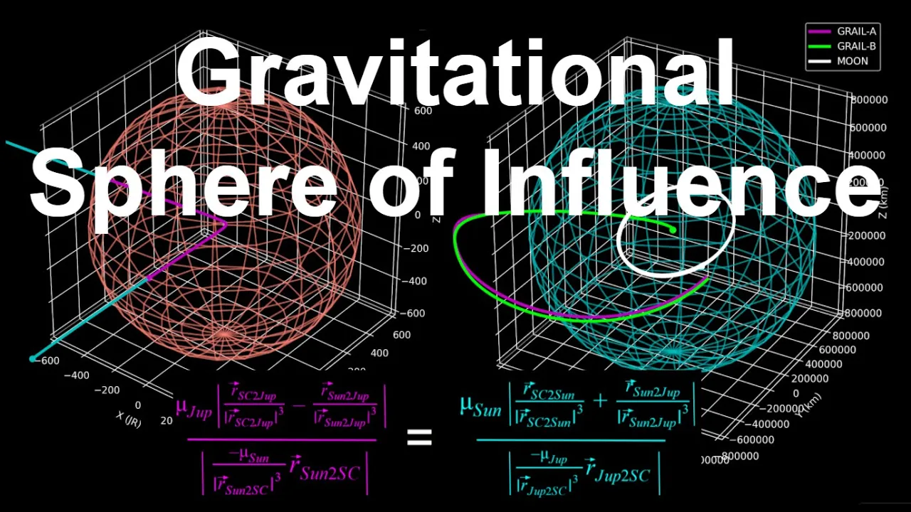
Why this video is valuable: This video addresses one of the major gaps highlighted in the review feedback: calculating a planet's Sphere of Influence (SOI). It explains the math behind the boundary where a planet’s gravity begins to dominate over solar gravity. It derives the Laplace limit equation $r_{SOI} \approx a \left(\frac{m}{M}\right)^{2/5}$ (where $a$ is the planet's semi-major axis, $m$ is the mass of the planet, and $M$ is the mass of the Sun) and demonstrates how to implement this programmatically in Python.

Gravity Assist (gravitational slingshot)

@Ingenium_dr05:09621

Gravity Assist (gravitational slingshot)

A gravity assist maneuver allows a spacecraft to increase its speed by flying by a moving planet, where the spacecraft gains velocity equal to twice the planet's velocity (VS2 = VS1 + 2*VP1) while the planet's velocity decreases by a negligible amount due to the spacecraft's much smaller mass.

@Ingenium_dr · 05:09

Why this video is valuable: This video bypasses standard popular-science simplifications to present the actual vector physics of a gravity assist. It explains how a spacecraft's hyperbolic excess velocity ($v_{\infty}$) relative to the flyby planet remains constant in magnitude but changes in direction. By transitioning this deflection vector into the heliocentric reference frame, it proves mathematically how a spacecraft gains or loses planet-relative orbital velocity without consuming any fuel.

Knowledge Checkpoint

• Explain the patched conics approximation and identify its three primary stages.
• Calculate the radius of Earth’s and Mars' Spheres of Influence (SOI) using the Laplace equation.
• Explain why the magnitude of the hyperbolic excess velocity vector ($|\vec{v}_{\infty, in}|$) must equal the outgoing magnitude ($|\vec{v}_{\infty, out}|$) in a planet's local reference frame during a gravity assist.
• Sketch the vector addition showing how passing behind a planet's orbital path increases a spacecraft's heliocentric velocity, while passing in front of it decreases it.

Module 5: The Three-Body Problem and Lagrangian Points

The classical two-body approximation fails to capture complex orbital regimes like those near Lagrange points. This module covers the Circular Restricted Three-Body Problem (CRT3BP), derives the equations of motion in a rotating coordinate system, and discusses the engineering applications of Lagrangian points (L1-L5), halo orbits, and Lissajous trajectories.

Recommended Videos

3-Body Problem Equations Derived, Part 2: Rotating Frame | Topic 3

@ProfessorRoss06:375,546

3-Body Problem Equations Derived, Part 2: Rotating Frame | Topic 3

Transforming gravitational forces to the rotating frame involves substituting r_N = A(τ)r_B into the gravitational equations. After algebraic manipulation, the complete equations of motion become autonomous ODEs: d²x/dτ² - 2dy/dτ - x = - (1-μ)(x + μ)/r₁³ + μ(x - (1-μ))/r₂³, with similar expressions for y and z components. The mass parameter μ determines system behavior and is the ratio of the smaller primary's mass to total mass. These equations describe the motion of a test particle under the g

@ProfessorRoss · 06:37

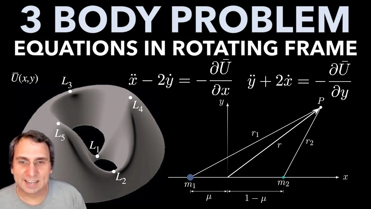
Why this video is valuable: This lecture resolves the math gap highlighted in the review feedback regarding the Circular Restricted Three-Body Problem (CRT3BP). It walks through the derivation of the equations of motion within a rotating coordinate system, introducing the Coriolis and centripetal terms that emerge from the coordinate system transformation. This is essential for understanding how Lagrange points are calculated.

The Lagrangian Points are Awesome... Tutorial

@dcaulf15:01113,351

The Lagrangian Points are Awesome... Tutorial

Lagrangian points are five specific locations in a two-body gravitational system (such as the Sun-Earth system) where objects can maintain the same orbital period as the larger body despite being at different distances; these points exist because the combined gravitational forces from both bodies create effective changes in the apparent mass that govern orbital motion, allowing objects at different radial positions to achieve synchronized orbital periods.

@dcaulf · 15:01

Why this video is valuable: This tutorial offers a comprehensive mathematical and conceptual breakdown of the five Lagrange points (L1-L5) in a two-body gravitational system. It demonstrates how these locations represent equilibrium solutions where the gravitational pulls of two massive bodies combine with centripetal force to keep a third small body at a constant relative position. It clearly identifies which points are stable (L4, L5) and which are unstable (L1, L2, L3).

Tracking the James Webb Space Telescope as it Heads to the L2 Point!

@Astronomy_Live03:30404,111

Tracking the James Webb Space Telescope as it Heads to the L2 Point!

The James Webb Space Telescope orbits L2 rather than being stationary at the point because L2 is not truly stable. Any slight deviation would cause the spacecraft to drift away. Instead, the telescope maintains a halo orbit around L2, which is more stable and controllable. The combined gravitational forces of the Sun and Earth work together to keep the telescope traveling with Earth around the Sun, completing one orbit per year despite being 1.5 million kilometers further from the Sun. This orbi

@Astronomy_Live · 03:30

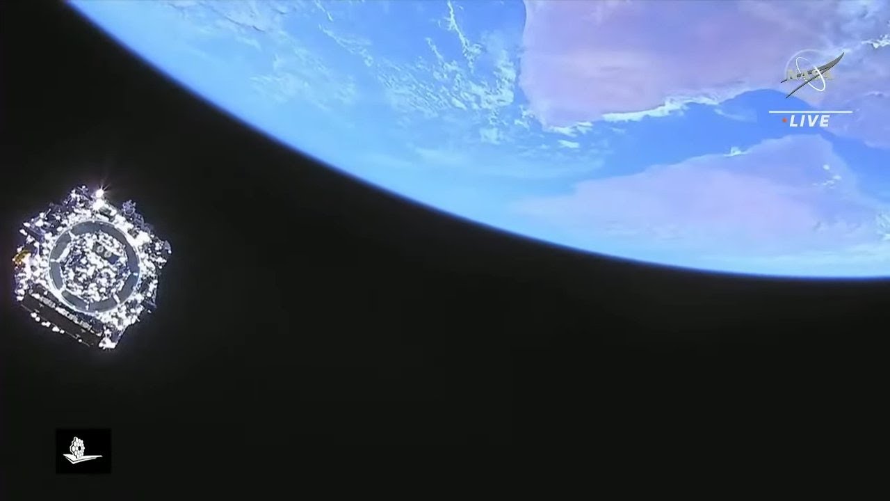
Why this video is valuable: Using the James Webb Space Telescope (JWST) as a case study, this video explains why spacecraft do not sit directly on an unstable Lagrange point like L2. Instead, they orbit "empty space" in a complex, three-dimensional halo orbit around L2. It details why this orbit requires active station-keeping and how it prevents Earth from eclipsing the telescope's vital solar panels.

Knowledge Checkpoint

• Write down the equations of motion for the Circular Restricted Three-Body Problem (CRT3BP) in a rotating reference frame, identifying the Coriolis and centrifugal acceleration terms.
• Locate the five Lagrange points in a system and explain the physical mechanisms balancing forces at each point.
• Explain why L1, L2, and L3 are unstable equilibrium points, while L4 and L5 can be dynamically stable under specific mass ratios ($m_1/m_2 > 24.96$).
• Define a halo orbit and explain why active station-keeping maneuvers are necessary for telescopes like JWST parked near the L2 point.

Course Map

Key People Index

• Johannes Kepler (1571–1630): German astronomer who formulated the three fundamental laws of planetary motion based on Tycho Brahe’s observational data, establishing that orbits are elliptical rather than circular.
• Sir Isaac Newton (1643–1727): English physicist and mathematician whose formulation of the laws of motion and universal gravitation provided the physical mechanics that derive Kepler's empirical laws.
• Joseph-Louis Lagrange (1736–1813): Italian-French mathematician who identified the five equilibrium points (Lagrange points) in the circular restricted three-body problem.
• Walter Hohmann (1880–1945): German engineer who proposed the coplanar transfer maneuver (Hohmann transfer) between two circular orbits, publishing the fuel-efficient orbital transit model in 1925.
• Gary Flandro (b. 1934): aerospace engineer who calculated the planetary alignment of the outer gas giants in the 1960s, discovering that gravity assists could be used to execute the "Grand Tour" multi-planet missions (ultimately realized in the Voyager 1 & 2 missions).
• Dr. Riccardo Bevilacqua: Professor of Aerospace Engineering (University of Florida), known for academic derivations of astrodynamics models and Newtonian mechanics applications.
• Alfonso Gonzalez: Astrodynamics software engineer specializing in orbital mechanics simulations, state estimations, and orbital math implementations using computational frameworks (Python).

Final Self-Assessment

Test your mastery of orbital mechanics and trajectory design by completing the tasks in this self-assessment checklist.

• Gravitational Derivation: Can you mathematically derive Kepler’s Third Law ($T^2 \propto a^3$) starting from Newton’s Law of Universal Gravitation and the equation for circular centripetal force?
• State Vector Transformations: Can you construct a rotation matrix to transform coordinate representations from the 3D perifocal plane coordinate system ($PQW$) back to the geocentric equatorial frame ($IJK$)?
• Hohmann Transfer Calculation: Given an initial low Earth circular orbit at $r_1 = 6778\text{ km}$ and a target geosynchronous circular orbit at $r_2 = 42164\text{ km}$, can you calculate the exact delta-v burn required at periapsis ($\Delta v_1$), apoapsis ($\Delta v_2$), and the transfer's total Time of Flight (TOF)?
• Bi-elliptic Superiority Limit: Can you mathematically prove or explain why a bi-elliptic transfer requires less delta-v than a Hohmann transfer if the ratio of the final circular orbit radius to the initial circular orbit radius exceeds $15.58$?
• Plane Change Economics: Can you calculate the delta-V required to adjust an Earth satellite's orbit inclination from $28.5^\circ$ to $0^\circ$ at an altitude of $300\text{ km}$ ($v \approx 7.73\text{ km/s}$), and explain how much delta-v is saved if the maneuver is postponed until the satellite reaches an apogee of $35786\text{ km}$ ($v \approx 1.6\text{ km/s}$)?
• Sphere of Influence Calculation: Can you compute the Sphere of Influence (SOI) radius of Jupiter relative to the Sun, using Jupiter’s orbital semi-major axis ($7.78 \times 10^8\text{ km}$) and its mass ratio to the Sun ($1/1047$)?
• Patched Conics Integration: Can you sketch a complete patched conics mission profile for a spacecraft traveling from Earth to Mars, highlighting where the reference frames transition (hyperbolic geocentric departure $\rightarrow$ heliocentric elliptic $\rightarrow$ hyperbolic areocentric capture)?
• Slingshot Velocity Boost: Can you construct a vector diagram showing how a spacecraft flying behind Jupiter gains orbital energy and heliocentric velocity, and compute the maximum hypothetical exit velocity of the spacecraft if the flyby is perfectly elastic?
• Three-Body Coordinate Rotation: Can you explain why a rotating coordinate system is used in the CRT3BP model, and identify how the Coriolis ($2\dot{y}$) and centrifugal ($x, y$) terms appear in the equations of motion?
• Lagrangian Stability Constraints: Can you mathematically or conceptually explain why the colinear Lagrange points L1, L2, and L3 are unstable while the triangular points L4 and L5 are stable in the Earth-Sun system?
• Halo Orbit Dynamics: Can you describe the primary physical forces balancing a spacecraft in a three-dimensional Lissajous or halo orbit around the unstable L2 point, and explain why constant station-keeping thruster burns are required?