ML Optimization: Calculus, Hessians & Gradients

Learning Goal: Mastering multivariable calculus, Hessian matrices, and gradient descent algorithms to formulate, analyze, and optimize loss landscapes for machine learning models.

• Prerequisites: High-school algebra and basic Python scripting. No prior calculus or linear algebra knowledge is assumed.
• Estimated Total Study Time: 35 Hours

---

Module 1: Single-Variable Calculus Foundations

This module introduces the foundational concepts of calculus. You will build an intuitive understanding of rates of change, the limit definition of a derivative, and standard differentiation rules. This lays the groundwork for high-dimensional gradient calculations.

Recommended Videos

Why this video: This video demystifies calculus by removing intimidating jargon. It explains the derivative through highly visual, step-by-step physical examples (such as moving vehicles and changing velocities), making the concept of an "instantaneous rate of change" accessible.

---

Why this video: This video connects geometric intuition to formal algebra. It explains how the slope of a secant line between two points evolves into the slope of a tangent line at a single point as the distance ($\Delta x$) approaches zero.

---

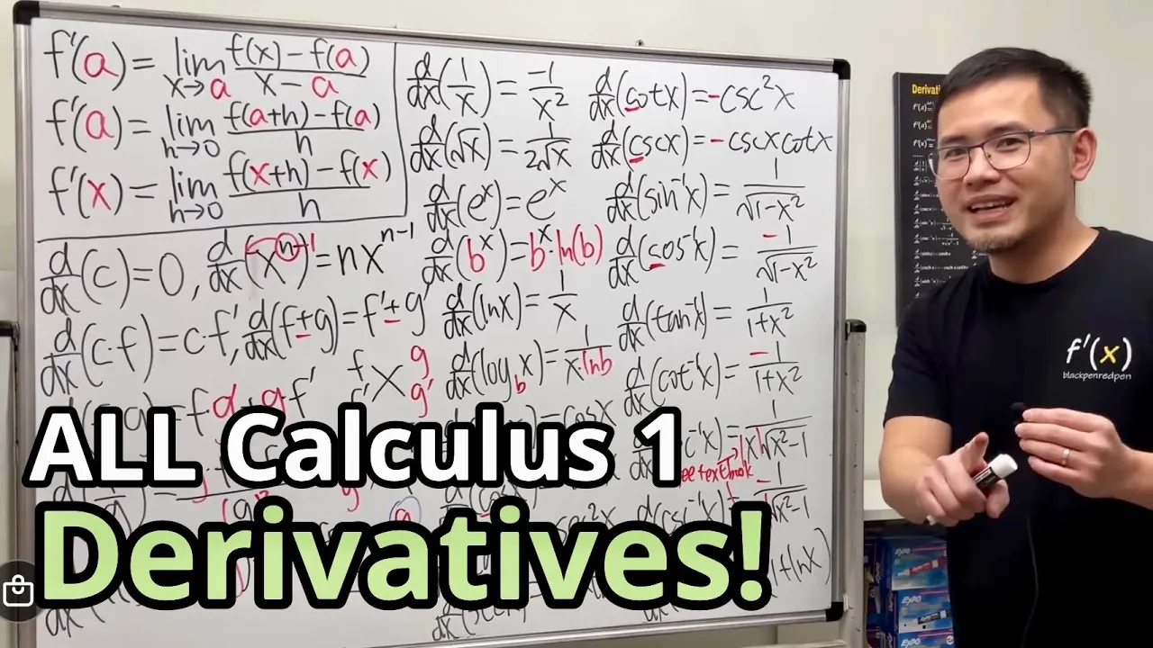
Why this video: To perform optimization, you must be comfortable computing derivatives manually. This video serves as a comprehensive reference guide, walking through the fundamental limit definition of the derivative and the core algebraic rules (Power Rule, Product Rule, Quotient Rule, and Chain Rule).

Calculus Foundations Study Note (Gap Correction): The video pool focuses heavily on applied rules and geometric intuition. For a deeper, rigorous mathematical analysis of limits and formal delta-epsilon proofs, we suggest independently searching for: "limit definition of derivative delta epsilon khan academy".

Knowledge Checkpoint

• Explain the difference between an average rate of change and an instantaneous rate of change.
• Derive the derivative of $f(x) = x^2$ using the limit definition: $\lim_{h \to 0} \frac{f(x+h) - f(x)}{h}$.
• State the Chain Rule and apply it to find the derivative of $f(x) = (3x^2 + 2x)^5$.

---

Module 2: Linear Algebra Foundations for Optimization

Machine learning models process high-dimensional datasets. In this module, you will master vectors, matrices, linear transformations, and the concepts of eigenvalues and eigenvectors. These tools allow you to analyze and navigate multi-dimensional loss landscapes.

Recommended Videos

Why this video: This video bridges the gap between physics, computer science, and mathematics. It demonstrates how vectors are not just lists of numbers, but arrows in space with length and direction that form the foundation of multidimensional math.

---

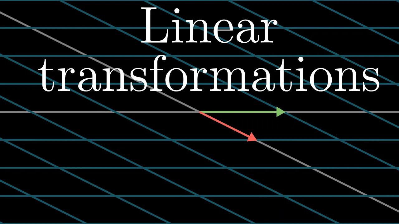
Why this video: This visual guide shows how matrices act as linear transformations that stretch, rotate, and deform coordinate space. Understanding this is key to visualizing how optimization algorithms transform loss landscapes.

---

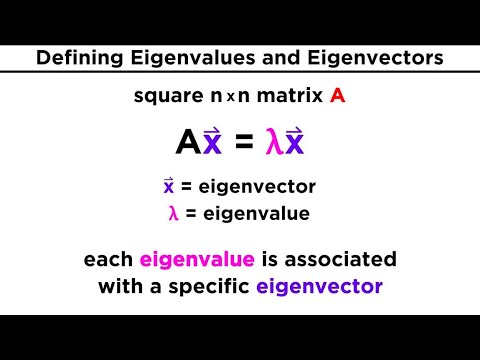
Why this video: Eigenvalues and eigenvectors reveal the directional characteristics of matrices. This tutorial explains the mathematics of solving the characteristic equation $\det(A - \lambda I) = 0$ to identify directions of pure scaling.

---

Why this video: This lecture reviews the exact matrix-vector notations used in ML literature. It covers transpose, dot product, Hadamard product (element-wise multiplication), and standard matrix multiplication.

Knowledge Checkpoint

• Graphically show how a $2 \times 2$ matrix transforms a unit grid.
• Define what makes a vector an eigenvector of a matrix $A$ and write the algebraic relationship.
• Given a $2 \times 2$ matrix, calculate its eigenvalues and find their corresponding eigenvectors.

---

Module 3: Multivariable Calculus & The Gradient Vector

This module extends calculus to functions of multiple variables. You will learn to compute partial derivatives, construct the gradient vector, and calculate directional derivatives to find paths of steepest descent.

Recommended Videos

Why this video: This video visualizes partial derivatives using 3D graphing software. It shows how holding one variable constant creates a 2D slice of a 3D surface, allowing you to compute a standard single-variable derivative along that slice.

---

Why this video: This video explains how the gradient vector ($\nabla f$) packages all the partial derivatives of a function. It shows mathematically why the gradient vector points in the direction of steepest ascent on a multi-dimensional surface.

---

Why this video: What if you want to move in a direction that isn't aligned with the coordinate axes? This video shows how to compute the rate of change along any arbitrary direction using the dot product of the gradient vector and a unit direction vector.

Knowledge Checkpoint

• Calculate the partial derivatives $\frac{\partial f}{\partial x}$ and $\frac{\partial f}{\partial y}$ for $f(x,y) = 3x^2y + \sin(x)e^y$.
• Explain why the gradient vector is always perpendicular (orthogonal) to the level curves of a function.
• Calculate the directional derivative of $f(x,y) = x^2 - y^2$ at the point $(1, 2)$ in the direction of the vector $\mathbf{v} = [3, 4]^T$.

---

Module 4: Jacobians, Hessians & Taylor Approximations

This module focuses on second-order relationships and multidimensional curves. You will study the Jacobian matrix (first-order changes in vector functions), the Hessian matrix (second-order curvature of scalar functions), and Taylor series approximations.

Recommended Videos

Why this video: This video explains the Jacobian matrix. It details how the Jacobian acts as a multidimensional transformation matrix, mapping small changes in input space to changes in output space for vector-valued functions.

---

Why this video: This video introduces the Hessian matrix, which organizes all second partial derivatives of a multivariable function. It shows how the Hessian measures multidimensional concavity, allowing you to identify local minima, local maxima, and saddle points.

---

Why this video: To approximate complex loss surfaces, we use Taylor series. This video details the formula for a quadratic approximation $Q(x,y)$ of a multivariable function, showing how the gradient and the Hessian are used to build the approximation.

---

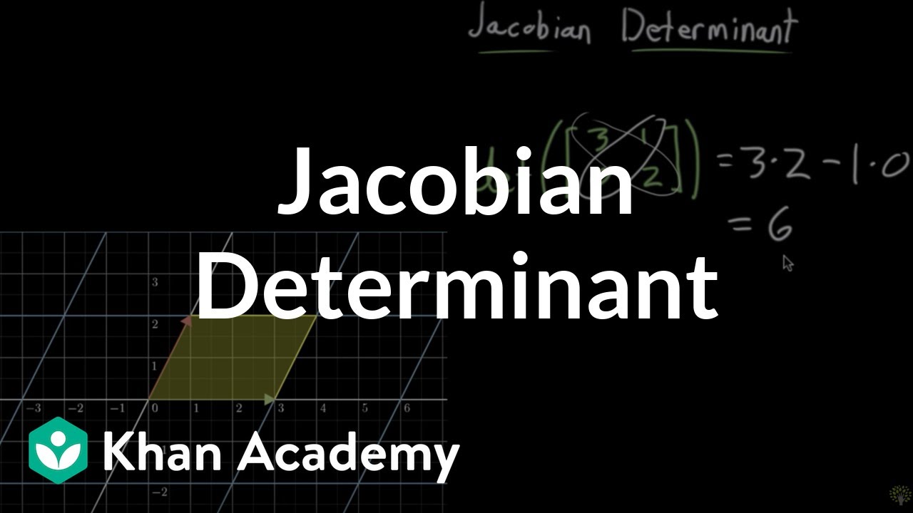
Why this video: This video explains how the determinant of the Jacobian measures local scaling. It shows how to calculate the factor by which a transformation stretches or compresses area in a neighborhood around a point.

Visualizing Multivariable Taylor Approximations (Gap Correction): While the videos above cover the algebra of quadratic approximations, visualizing these 3D Taylor approximations can be challenging. We recommend searching online for: "multivariable taylor series approximation visualization 3blue1brown" or "jacobian matrix intuitive explanation 3blue1brown" to see interactive animations.

Knowledge Checkpoint

• For a function $f: \mathbb{R}^n \to \mathbb{R}^m$, write out the general dimensions and structural entries of its Jacobian matrix.
• Construct the Hessian matrix for the function $f(x,y) = x^3 - 3xy + y^3$.
• Write out the multivariable quadratic Taylor expansion formula of $f(\mathbf{x})$ around a reference point $\mathbf{x}_0$.

---

Module 5: Gradient Descent & First-Order Optimization

This module covers first-order optimization. You will learn the mechanics of the gradient descent algorithm, analyze the role of the learning rate, and study how neural networks use backpropagation to calculate gradients.

Recommended Videos

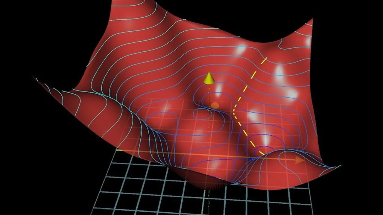
Why this video: This video provides a visual explanation of how neural networks learn. It frames gradient descent as a ball rolling down a hilly cost landscape, showing how calculating the negative gradient updates parameters to minimize error.

---

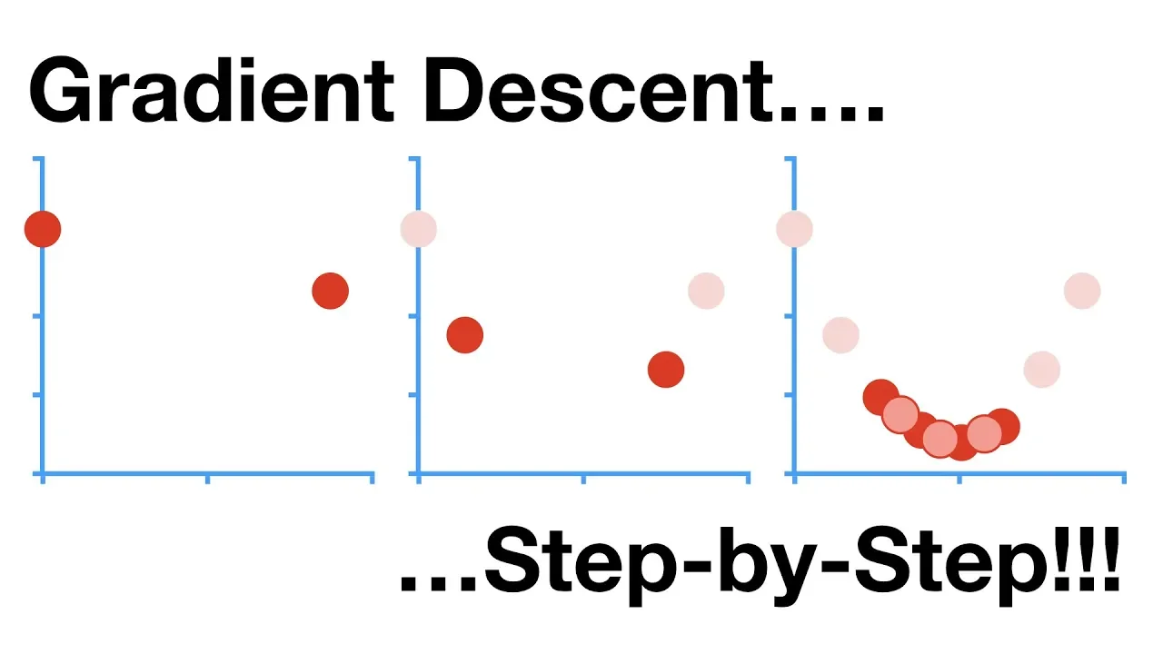
Why this video: This step-by-step tutorial demystifies the arithmetic of gradient descent. It shows how the chain rule is used to compute the slope of a loss function relative to intercept and slope parameters in regression models.

---

Why this video: This video analyzes the learning rate parameter ($\alpha$). It explains the consequences of choosing a learning rate that is too small (slow, expensive convergence) versus one that is too large (divergence, oscillation, and missing the minimum).

Knowledge Checkpoint

• Write down the parameter update formula for gradient descent, defining each symbol.
• Explain the relationship between the magnitude of the gradient vector and the step size as the algorithm approaches a local minimum.
• Sketch how gradient descent behaves on a loss surface when the learning rate is set too high.

---

Module 6: Advanced ML Optimizers & Second-Order Methods

This final module covers advanced optimization algorithms. You will study stochastic gradient descent (SGD), adaptive optimizers like RMSprop and Adam, and second-order optimization using Newton’s Method.

Recommended Videos

Why this video: This lecture from Stanford explores optimization challenges in deep learning. It explains why standard gradient descent struggles with ill-conditioned loss surfaces, gets stuck in saddle points, and how momentum and adaptive learning rates help address these issues.

---

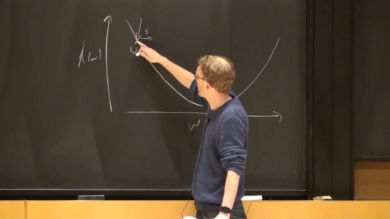
Why this video: This video contrasts first-order optimization with Newton's Method (a second-order approach). It demonstrates how Newton's method uses Hessian-derived curvature to calculate the ideal step size and direction, converging in fewer iterations.

---

Why this video: This video covers the mathematical formulation of multidimensional Newton's Method. It details the step-by-step application of the update rule $\mathbf{x}_{k+1} = \mathbf{x}_k - H(\mathbf{x}_k)^{-1} \nabla f(\mathbf{x}_k)$ and walks through a manual calculation.

---

Why this video: This technical lecture details the mathematical formulation of adaptive learning algorithms, covering SGD with momentum, RMSprop, and Adam. It explains how tracking historical gradients dynamically scales learning rates for each parameter.

The Hessian Computational Bottleneck (Gap Correction): While second-order methods offer faster mathematical convergence, they are rarely used in deep learning. A critical concept to study is the Curse of Dimensionality inverting the Hessian. For a model with $N$ parameters, the Hessian is an $N \times N$ matrix. Inverting this matrix requires $O(N^3)$ calculations, which is computationally prohibitive when $N$ is in the millions or billions. To learn more about this limit, search online for: "why we don't use newton's method in deep learning optimization".

Knowledge Checkpoint

• Explain how SGD with momentum prevents the optimization path from oscillating in steep, narrow valleys.
• Compare Newton's Method with gradient descent, detailing the advantages and disadvantages of each.
• Given a model with 1,000,000 parameters, compute the memory footprint of storing its Hessian matrix (using 32-bit floating point numbers) and explain why this makes inverting the matrix difficult.

---

Course Map

This flowchart shows the dependency structure of the modules. You should complete the foundational modules (Modules 1 and 2) before moving on to multivariable calculus and optimization algorithms.

---

Key People Index

• Sir Isaac Newton & Gottfried Wilhelm Leibniz (Module 1): Independent co-discoverers of calculus. Newton framed derivatives around physics and motion, while Leibniz developed the notation ($\frac{dy}{dx}$ and $\int$) used in modern calculus.
• Grant Sanderson (3Blue1Brown) (Modules 2 & 5): A math educator known for visual explanations of complex topics. His animations help develop visual intuition for linear algebra, calculus, and neural network learning.
• Josh Starmer (StatQuest) (Module 5): A biostatistician and educator who explains machine learning algorithms by breaking them down into step-by-step visual calculations.
• Kilian Weinberger (Cornell University) (Module 6): A prominent machine learning researcher whose lectures connect optimization theory to practical machine learning implementations.

---

Final Self-Assessment

This comprehensive assessment covers the core concepts from the entire curriculum. Complete this checklist to verify your understanding of ML optimization.

• Limit Interpretation: I can explain how the derivative represents a limit of secant slopes geometrically and algebraically.
• Matrix Transformations: I understand how a matrix scales space, and how to find eigenvectors that do not change direction during this transformation.
• Gradient Descent Optimization: I can mathematically prove why the negative gradient $-\nabla f(\mathbf{x})$ points in the direction of steepest descent.
• Linear vs. Directional Derivatives: I can explain the difference between a partial derivative and a directional derivative, and calculate both.
• The Jacobian Role: I can construct the Jacobian matrix for vector-valued functions and explain its role in computing backpropagation gradients.
• Hessian Curvature: I can construct a Hessian matrix and use its eigenvalues to classify a critical point as a local minimum, local maximum, or saddle point.
• Taylor Approximations: I can write out a multivariable quadratic approximation and explain how it models a complex loss landscape locally.
• Hyperparameter Effects: I understand how the learning rate ($\alpha$) affects convergence, and can identify signs of under-shooting and over-shooting.
• Modern Optimizers: I can explain the differences between vanilla SGD, Momentum, RMSprop, and Adam.
• Second-Order Limitations: I can explain why Newton's Method is rarely used directly in deep learning models due to the computational cost of inverting the Hessian matrix.