Projective Geometry: Coordinates & Conics
Learning Goal: Transition from classical Euclidean space to projective space using homogeneous coordinates, understand the algebraic elegance of duality, master the projective invariance of cross-ratios, and classify conic sections under projective transformations.
Projective geometry simplifies our understanding of space by eliminating special cases like parallel lines and infinite limits. By treating "infinity" as a tangible geometric location, it provides a unified mathematical framework vital for fields ranging from algebraic geometry to computer vision and computer graphics.
Prerequisites
- Linear Algebra: Vector spaces, basis transitions, linear transformations, matrix multiplication, determinants, and eigenvalues.
- Analytical Geometry: Cartesian coordinate representation of lines, planes, and conic sections (ellipses, parabolas, hyperbolas).
Estimated Study Time
- Total Course Duration: ~14 Hours (including video lectures, supplementary reading, and mathematical derivations).
Module 1: From Euclidean to Projective Space
This module bridges the gap between Euclidean geometry and projective geometry. You will study how painters during the Renaissance discovered the mathematical laws of perspective, why parallel lines intersect at a "vanishing point" (point at infinity), and how the real projective plane is topologically constructed.
Recommended Videos

- Why this video: This academic lecture from Oxford University provides a rigorous mathematical introduction to the projective plane. It formally extends affine space by introducing points at infinity, demonstrating how any two distinct lines in a projective plane intersect at exactly one point, thus removing the exceptional case of parallel lines.
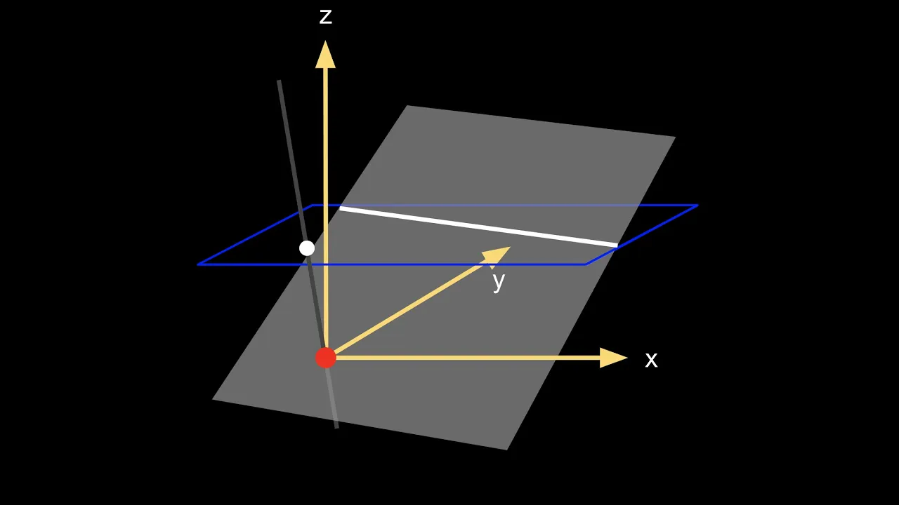
- Why this video: It bridges geometric intuition with the language of linear algebra, explaining how a 3D vector space can represent the 2D projective plane. This visual foundation makes the subsequent transition to algebraic notation highly intuitive.

- Why this video: A brief overview of why projective geometry is more fundamental than Euclidean geometry. It emphasizes that projective space relies on fewer baseline assumptions (such as the absence of metrics or angles) and highlights its focus on incidence properties.
- Why this video: This lecture explores the historical and visual origins of projective geometry through Renaissance perspective art. It details how polymaths like Filippo Brunelleschi and Piero della Francesca formalized the concept of the vanishing point mathematically.
Module 1 Knowledge Checkpoint
- Understand how projective space eliminates the parallel postulate by introducing ideal points.
- Describe the topological construction of the real projective plane (e.g., identifying antipodal points on a sphere).
- Articulate how perspective projections project 3D scenes onto 2D planes, and identify what geometric properties are preserved vs. lost.
Module 2: Homogeneous Coordinates
To compute inside projective space, we must move past Cartesian coordinates. In this module, you will learn to represent points and lines using homogeneous coordinates, mapping 2D Cartesian points to 1D equivalence classes in . This conversion allows for the elegant algebraic representation of points and lines at infinity.
Recommended Videos

- Why this video: A precise and compact explanation of how the 2D projective plane is constructed using 3D coordinates. It explains the mapping of normal affine points () and points at infinity (), illustrating why the zero vector is excluded.

- Why this video: This video focuses on the core equivalence relationship of homogeneous coordinates, demonstrating that scaling a point vector by any non-zero constant preserves the underlying projective point.
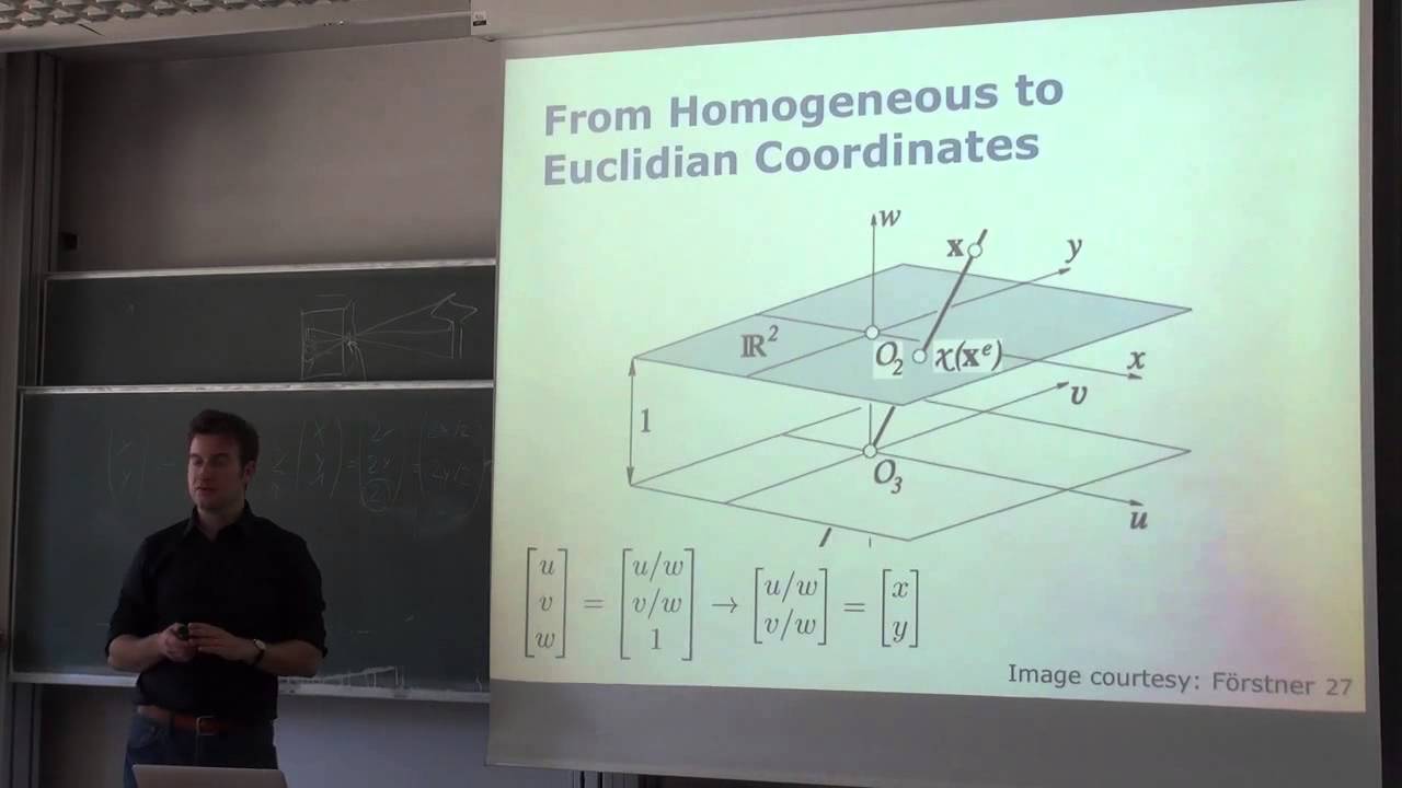
- Why this video: This lecture explains the engineering and scientific motivations behind using homogeneous coordinates. It illustrates how traditional Euclidean metrics cause division-by-zero errors when dealing with projections at infinity, and shows how homogeneous coordinates resolve this issue.

- Why this video: A rigorous, graduate-level deep dive into homogeneous coordinate systems. It explains the transformation pipelines used in robotics and photogrammetry, providing the linear algebraic machinery needed to manipulate matrices in projective space.
Module 2 Knowledge Checkpoint
- Convert 2D Cartesian points to homogeneous coordinates and vice versa.
- Define the line at infinity and explain why any point at infinity lies on it.
- Algebraically calculate the intersection of two parallel lines using the cross product of their homogeneous line vectors.
- Explain why scaling all homogeneous elements by a non-zero constant does not alter the geometric representation.
Module 3: Duality and Projective Transformations
Here, we explore the deep algebraic symmetries of the projective plane. First, we examine the Principle of Duality, where points and lines are represented by identical 3-component vectors, making them entirely interchangeable in geometric theorems. Second, we study Homographies—the matrices that define projective transformations (collineations) of .
Recommended Videos

- Why this video: Although brief, this video demonstrates the duality mapping in action, showing how a primal theorem regarding points and lines corresponds directly to a dual theorem where those structures swap roles.
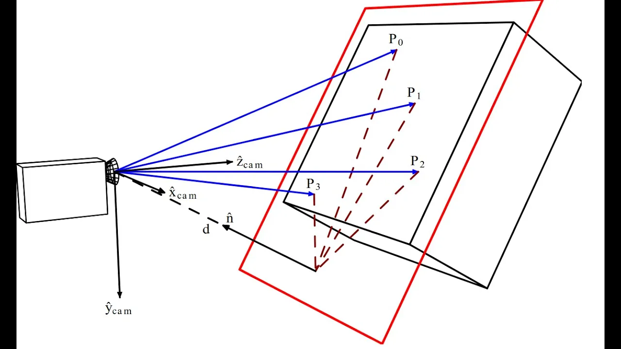
- Why this video: This video provides an intuitive and practical explanation of homography matrices (), which map points from one plane to another. It details how the 8 degrees of freedom of the projective matrix are solved using point correspondences.

- Why this video: This short lecture extract explains the hierarchy of geometric transformations, positioning projective transformations (homographies) as the most general class. It highlights that homographies have 9 entries but only 8 degrees of freedom due to scale ambiguity.
Deep-Dive: The Mathematics of Projective Duality
Because video coverage on the mathematical mechanics of duality can be sparse, study this formulation carefully:
In the projective plane , a point and a line are both represented as 3-vectors: A point lies on a line if and only if their inner product is zero: This equation is entirely symmetric. If you swap the vectors and , the algebraic statement is identical.
Consequently:
- Intersection of two lines: The point of intersection of two lines and is given by their cross product: .
- Line through two points: Dual to the above, the line passing through two points and is given by their cross product: .
Every valid geometric theorem in projective space has an immediate dual theorem obtained by exchanging the words "point" and "line", "intersection" and "join", and "collinear" and "concurrent".
Module 3 Knowledge Checkpoint
- State the Principle of Duality and explain how points and lines correspond.
- Prove why the cross product of two homogeneous line representations yields their point of intersection.
- Construct a homography matrix and explain why it has 8 degrees of freedom instead of 9.
- Transform a line under a homography , demonstrating that the line transforms as .
Module 4: Cross-Ratios and Projective Invariants
While angles, lengths, and parallelisms are lost under projective transformations, one fundamental metric property remains perfectly preserved: the cross-ratio of four collinear points. This module introduces the cross-ratio, its invariance under homographies, and its application to harmonic division and harmonic bundles.
Recommended Videos
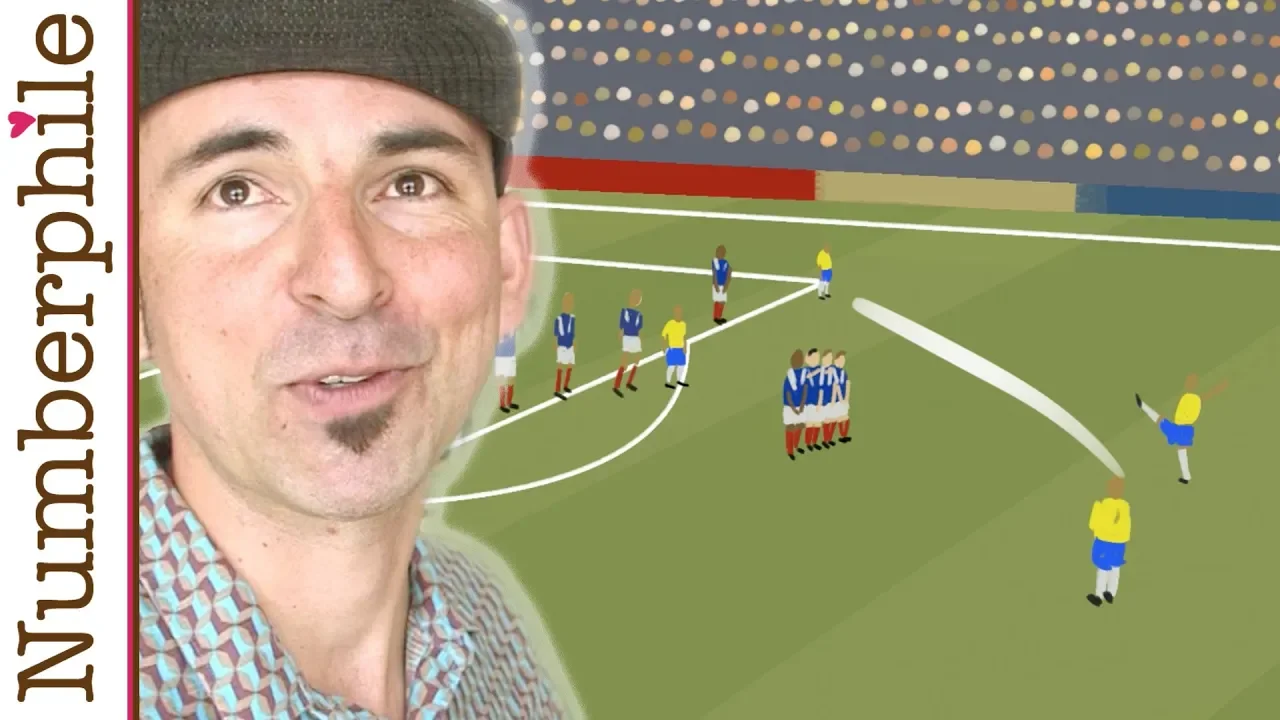
- Why this video: An exceptionally clear, visual, and intuitive introduction to the cross-ratio. Using real-world examples (like analyzing camera perspective distortions in photographs), it explains why this specific ratio remains constant regardless of the camera's angle or focal length.

- Why this video: This lecture links the cross-ratio to complex analysis and Möbius transformations on the Riemann sphere (which is projectively isomorphic to ). It proves the invariance of the cross-ratio under projective mappings.

- Why this video: This video focuses on solving advanced geometry problems using harmonic bundles. It shows how to identify four collinear points whose cross-ratio is exactly , a concept known as harmonic division.
Mathematical Supplement: Harmonic Bundles
A harmonic bundle is a set of four collinear points whose cross-ratio is defined as: Geometrically, this represents a highly symmetric division of a line segment. If divides the segment internally in a ratio of , then divides externally in the same ratio .
A C B D
-------------------------------------------------->
In any projective drawing, if you construct a complete quadrangle (a 4-point frame), its diagonals and intersection points automatically project to a harmonic bundle on any intersecting line. This geometric construction allows you to locate the harmonic conjugate of a point relative to and using only an unmarked straightedge.
Module 4 Knowledge Checkpoint
- Compute the cross-ratio for a given set of four collinear points.
- Prove analytically that any 1D projective transformation preserves the cross-ratio.
- Define a harmonic bundle and construct one geometrically using a complete quadrangle.
- Calculate the position of a harmonic conjugate point both in Cartesian coordinates and using homogeneous representations.
Module 5: Projective Conic Sections
In Euclidean geometry, circles, ellipses, parabolas, and hyperbolas are distinct curves with different formulas. In projective geometry, all non-degenerate conic sections are projectively equivalent. This module explores the projective classification of conics and introduces the projective polar theory—the geometric relationship between a point (pole) and a line (polar) relative to a conic.
Recommended Videos

- Why this video: A comprehensive lecture detailing conics in projective 2D space. It explains how quadratic equations in homogeneous coordinates are represented by symmetric matrices () and details why non-degenerate conics are equivalent.
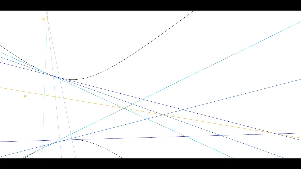
- Why this video: This video explains pole and polar theory. It shows how a pole point relates to its polar line with respect to a conic section, illustrating the construction using harmonic ranges and secant lines.
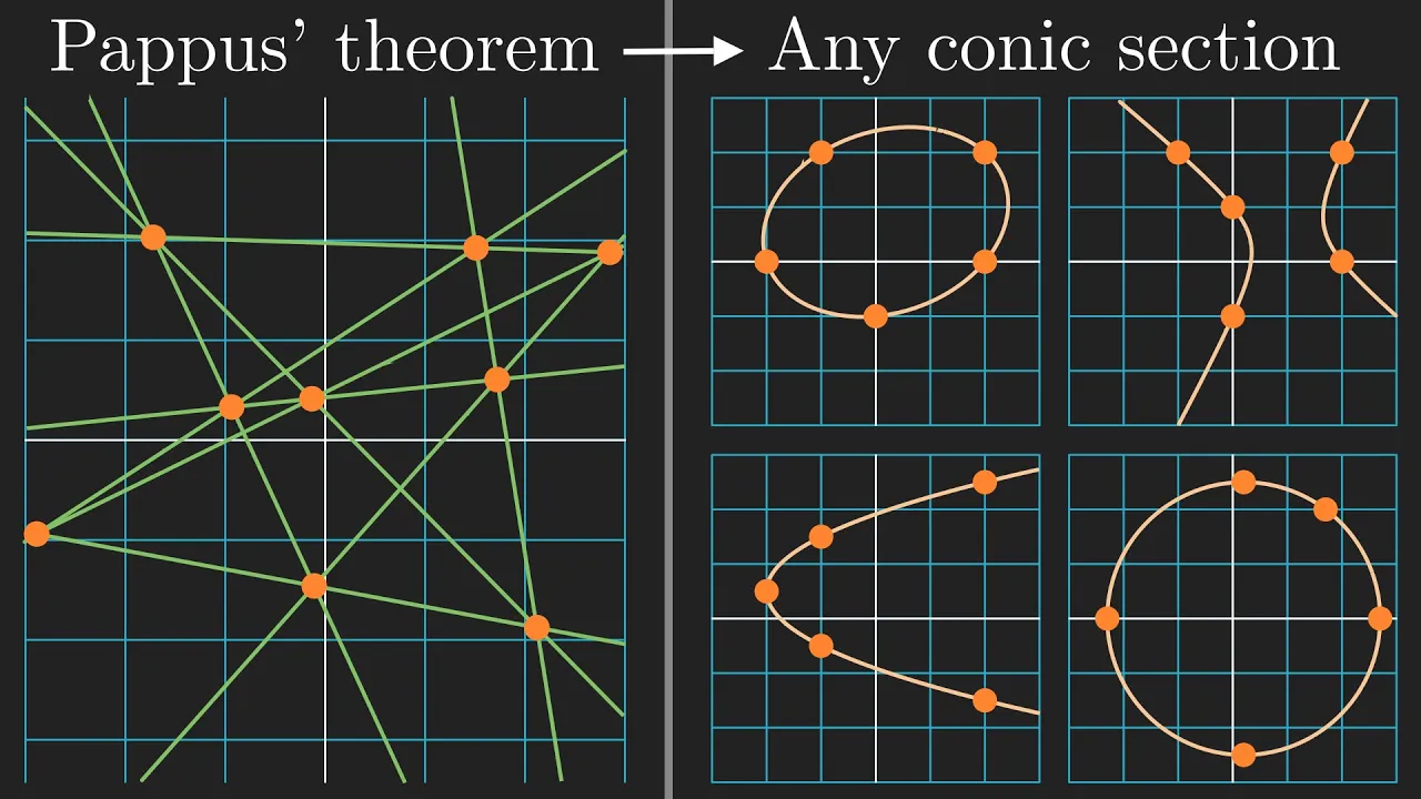
- Why this video: Combining projective theorems (specifically Pappus' and Pascal's theorems), this video demonstrates how five arbitrary points in projective space uniquely define a conic section, illustrating the coordinate-free visual beauty of conic projections.

- Why this video: Offers a practical mathematical walkthrough for computing poles and polars. Although framed around circles, the underlying linear algebra directly maps to projective conics via the matrix product .
Projective Classification vs. Euclidean Graphing
Crucial Study Guide Note: When studying this module, avoid high-school level tutorials focused on graphing parabolas or finding Euclidean foci. In projective space, conics are classified by their signature (eigenvalues of the symmetric conic matrix ).
A real, non-degenerate conic in projective space is represented as: where is a symmetric matrix. Since all real symmetric matrices can be diagonalized, they can be transformed via a homography such that the conic becomes: This means that an ellipse, a parabola, and a hyperbola are simply different affine "slices" of this single projective conic. The differences we see in Euclidean space depend entirely on how the conic intersects the line at infinity :
- Ellipse: Does not intersect (contains only complex intersection points).
- Parabola: Is tangent to at exactly one point.
- Hyperbola: Intersects at two distinct real points (which define its asymptotes).
Module 5 Knowledge Checkpoint
- Write a conic section in projective coordinates as a symmetric matrix equation .
- Explain why ellipses, parabolas, and hyperbolas are projectively equivalent.
- Compute the polar line of a given pole point relative to a conic using the relationship .
- Use Pascal's Theorem to explain why 5 coplanar points are sufficient to uniquely identify a conic section.
Course Map
Key People Index
- Filippo Brunelleschi (1377–1446): Italian architect and designer who formulated the first mathematical rules of linear perspective, setting the foundation for projective space.
- Piero della Francesca (1415–1492): Renaissance painter and mathematician who wrote De Prospectiva Pingendi, the earliest scientific treatise on perspective drawing.
- Jean-Victor Poncelet (1788–1867): French engineer and mathematician who revived projective geometry as an independent field of study during his time as a prisoner of war. He formalized the Principle of Duality and the projective properties of conics.
- Menaechmus (380–320 BC): Ancient Greek mathematician credited with discovering conic sections while trying to solve the "doubling the cube" problem.
Final Self-Assessment
Test your mastery of the complete curriculum by completing this comprehensive evaluation:
- Can you define the fundamental topological differences between the affine plane and the real projective plane ?
- Can you transition a system of parallel lines in Cartesian coordinates to homogeneous form and prove that their intersection point lies on the line at infinity ?
- Given a line and a point in projective space, can you verify whether the point lies on the line?
- Can you explain the geometric meaning of the dual statement: "The dual of three collinear points is three concurrent lines"?
- Can you compute the Homography matrix mapping four known coplanar points to four target points using the Direct Linear Transformation (DLT) method?
- Can you write down the algebraic formula for the cross-ratio of four points and show that it does not change when the points are scaled by different homogeneous factors?
- Can you construct a harmonic bundle and identify the harmonic conjugate of the origin relative to two fixed coordinates?
- Can you prove why a parabola can be mapped to a circle using a projective transformation, and describe which projection centers are required to make this transformation?
- For a conic represented by matrix , if you are given a line , can you analytically calculate its pole ?