TDA: Simplicial Complexes & Homology

Learning Goal: Topological Data Analysis (TDA): Mapping the shape of data using simplicial complexes, persistent homology, and barcode visualizations.

• Prerequisites: Basic high-school algebra and an introductory understanding of coordinate geometry. No prior knowledge of topology, advanced abstract algebra, or coordinate-free linear algebra is required.
• Estimated Total Study Time: 16 Hours (including video lectures, recommended mathematical exercises, and coding environment setup).

---

Module 1: Foundations: Intuitive Topology & Linear Algebra

Module Overview

To understand how we can extract shapes and structures from coordinates, we must first establish a mathematical baseline. This module covers the intuitive mechanics of "rubber-sheet geometry" (topology), the precise definition of vector spaces (which will allow us to compute homology algebraically), and the fundamentals of group theory. We will focus on how abstract algebra strips away superficial properties to study structures via symmetric operations and invariants.

Recommended Videos

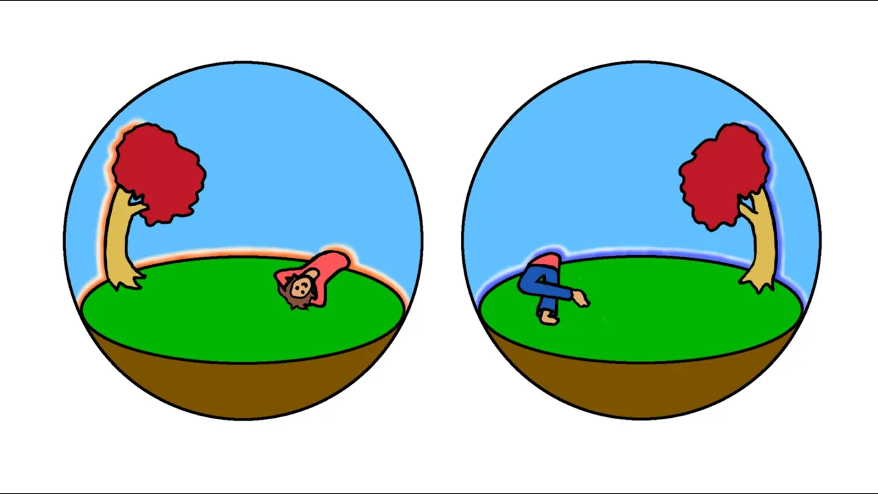
• Why this video is valuable: It strips away the intimidating jargon of point-set topology to build an intuitive mental model of objects as infinitely stretchable rubber. It clearly explains the rules of continuous deformation (stretching, bending, and twisting without tearing or gluing), paving the way for topological invariants.

---

• Why this video is valuable: This lecture introduces vector spaces using Sheldon Axler's rigorous, linear-map-first approach. Because topological homology calculations rely on treating chains of simplices as vector spaces, mastering the definition of fields, closure, and vector spaces over fields is critical.

---

• Why this video is valuable: Homology groups are the central mathematical tool of TDA. This lecture defines a group and its axioms (closure, associativity, identity, and inverses) using integers under addition. This foundational knowledge is essential for understanding the transition to free abelian groups and homology classes.

Knowledge Checkpoint

• Can you define a homeomorphism and explain why a coffee cup is topologically equivalent to a donut, but not to a sphere?
• What are the eight axioms of a vector space over a field $\mathbb{F}$?
• Why is the set of integers $\mathbb{Z}$ under addition a group, while the set of integers under multiplication is not?

---

Module 2: Simplicial Complexes: Building Shapes from Data

Module Overview

Point clouds (raw data points) do not have topological features on their own; they are simply disjoint collections of points. To measure their shape, we must construct combinatorial frameworks called simplicial complexes. This module details how to assemble points (0-simplices), edges (1-simplices), triangles (2-simplices), and tetrahedra (3-simplices) to model data. Additionally, we analyze the critical differences between the Čech complex and the computationally efficient Vietoris-Rips complex.

Recommended Videos

• Why this video is valuable: Professor Melvin Leok defines simplicial complexes from a combinatorial and geometric standpoint. He explains how simplices must glue together along shared faces and outlines the closed-under-inclusion property of abstract simplicial complexes.

---

• Why this video is valuable: This video resolves a common gap in TDA studies by explicitly comparing Čech and Vietoris-Rips complexes. It details why the Čech complex preserves the true homotopy of union-of-balls constructions (via the Nerve Theorem) while showing how the Rips complex relaxes these intersection rules to gain computational efficiency.

---

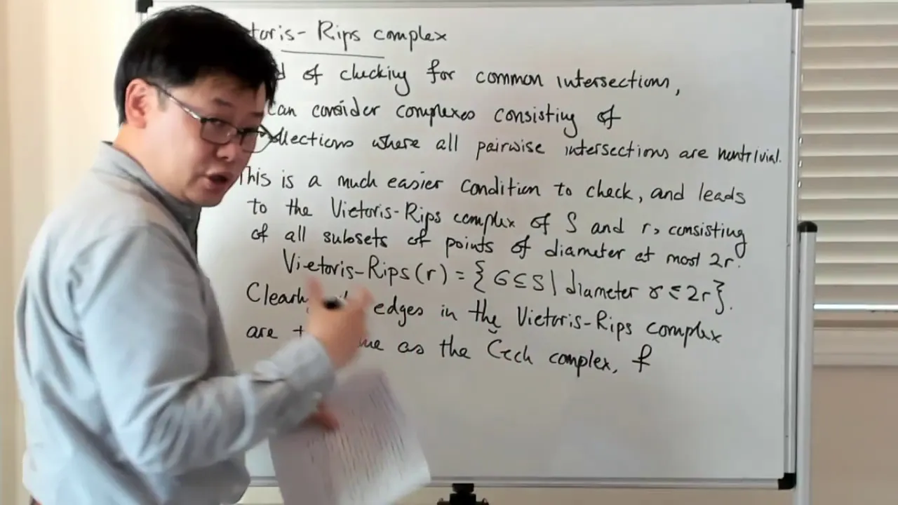
• Why this video is valuable: This lecture focuses on the mechanics of building a Vietoris-Rips complex. It demonstrates how to determine if higher-dimensional simplices should be added to a graph based solely on pairwise distances, highlighting its usefulness for algorithmic implementations.

Knowledge Checkpoint

• What is the formal definition of an abstract simplicial complex? If $\{v_0, v_1, v_2\}$ is in the complex, which other subsets must also be in it?
• What is the Nerve Theorem, and why does it guarantee that the Čech complex matches the topology of the union of open balls?
• Given three points forming an equilateral triangle of side length $d$, at what radius parameter $r$ does a 2-simplex (the solid triangle) form in the Vietoris-Rips complex versus the Čech complex?

---

Module 3: Homology: Measuring Holes in Data

Module Overview

With our simplicial complexes constructed, we need a mathematical tool to systematically count their structural "holes." This is the role of homology. In this module, we construct chain groups, define the boundary operator (which maps a simplex to its boundary), and show that "boundaries have no boundary" ($\partial^2 = 0$). This key algebraic fact allows us to divide cycles by boundaries to calculate Betti numbers, which count connected components ($\beta_0$), 1D loops ($\beta_1$), and 2D voids ($\beta_2$).

Recommended Videos

• Why this video is valuable: This video provides a highly visual explanation of homology. It shows how algebraic topology distinguishes between closed paths (cycles) that enclose a physical empty space (holes) and those that wrap around filled-in regions (boundaries).

---

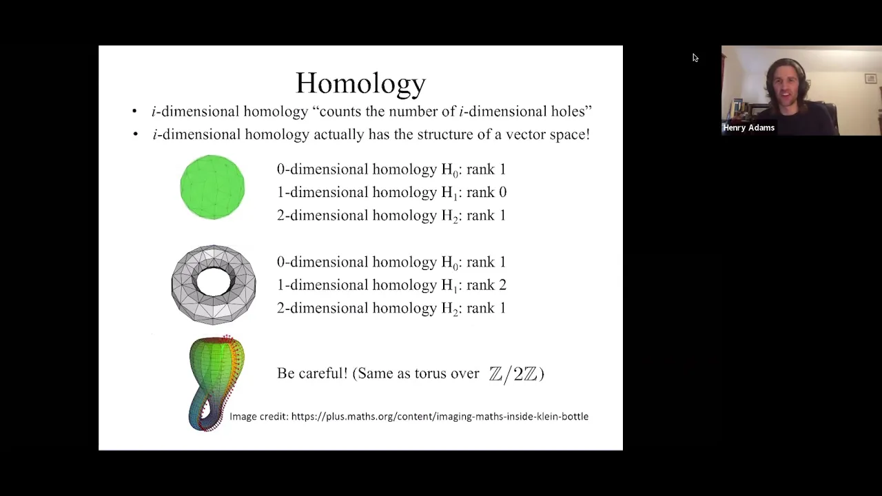
• Why this video is valuable: This video formalizes Betti numbers ($\beta_0, \beta_1, \beta_2$) and explains homology using vector spaces with coefficient fields like $\mathbb{Z}_2$. It connects topological intuition directly to linear algebra.

---

• Why this video is valuable: This lecture provides a clear derivation of the boundary operator ($\partial$) acting on an oriented $k$-simplex. It walks through the alternating sum formula $\partial[p_0, \dots, p_k] = \sum (-1)^i [p_0, \dots, \hat{p}_i, \dots, p_k]$ and explains why applying this boundary operator twice yields zero ($\partial_{k-1} \circ \partial_k = 0$).

Knowledge Checkpoint

• Write down the boundary operation $\partial_2$ on a oriented 2-simplex $[v_0, v_1, v_2]$. Show that $\partial_1(\partial_2[v_0, v_1, v_2]) = 0$.
• Define the $k$-th homology group $H_k(K)$ in terms of the kernel of $\partial_k$ (cycles $Z_k$) and the image of $\partial_{k+1}$ (boundaries $B_k$).
• What physical structures in a 3D dataset are measured by Betti numbers $\beta_0$, $\beta_1$, and $\beta_2$?

---

Module 4: Persistent Homology: Analyzing Across Scales

Module Overview

In real-world data, choosing a single radius parameter $r$ to construct a simplicial complex is problematic: too small, and the data looks like disconnected noise; too large, and it collapses into a single solid shape. Persistent homology solves this by analyzing all scales simultaneously. We grow balls around data points, creating a nested sequence of simplicial complexes called a filtration. By tracking when topological features are born and when they die, we can distinguish stable structural features from short-lived noise. We will also learn the column-reduction algorithm used to compute these persistence intervals from boundary matrices.

Recommended Videos

• Why this video is valuable: A clear introduction to the concept of filtrations. It shows how nested complexes preserve inclusion maps, allowing us to track topological features as the scale parameter changes.

---

• Why this video is valuable: This video bridges a major educational gap in TDA: understanding the actual mechanics of persistent homology computations. Henry Adams works through an explicit example, showing how to order simplices to build a boundary matrix and determine births and deaths.

---

• Why this video is valuable: This lecture explains the core column-reduction algorithm used in TDA software. It details the left-to-right elimination process on boundary matrices, explaining how to resolve column conflicts to find the pivots that mark the births and deaths of topological features.

Knowledge Checkpoint

• What is a filtration of a simplicial complex? Why must the complexes satisfy $K_0 \subseteq K_1 \subseteq \dots \subseteq K_n$?
• How does the boundary matrix reduction algorithm identify whether a simplex creates (birth) or destroys (death) a topological feature?
• If a topological feature has a birth time of $t=1.2$ and a death time of $t=1.5$, what is its persistence? Is it likely to be structural signal or noise?

---

Module 5: Barcodes & Applications: TDA in Practice

Module Overview

Once we calculate our birth and death points, we need to visualize and interpret them. This module covers Persistence Barcodes and Persistence Diagrams, explaining how to read them and how to measure differences between them using bottleneck and Wasserstein distances.

We will also look at how to run these analyses in Python. While YouTube has limited video coverage on libraries like GUDHI and Ripser, we will use Elizabeth Munch's tutorial as a starting point. We will also outline how to set up and run a standard TDA workflow in Python to analyze point cloud data.

Recommended Videos

• Why this video is valuable: Henry Adams compares the two primary ways to visualize persistent homology: horizontal barcodes (ordered by birth and death) and persistence diagrams (where birth and death are plotted as coordinates on a 2D plane). He also explains the diagonal line ($y=x$) on these diagrams.

---

• Why this video is valuable: A quick introduction to Python-based TDA. It shows how alternative filtration methods construct nested structures, illustrating how theoretical concepts translate into computational code.

---

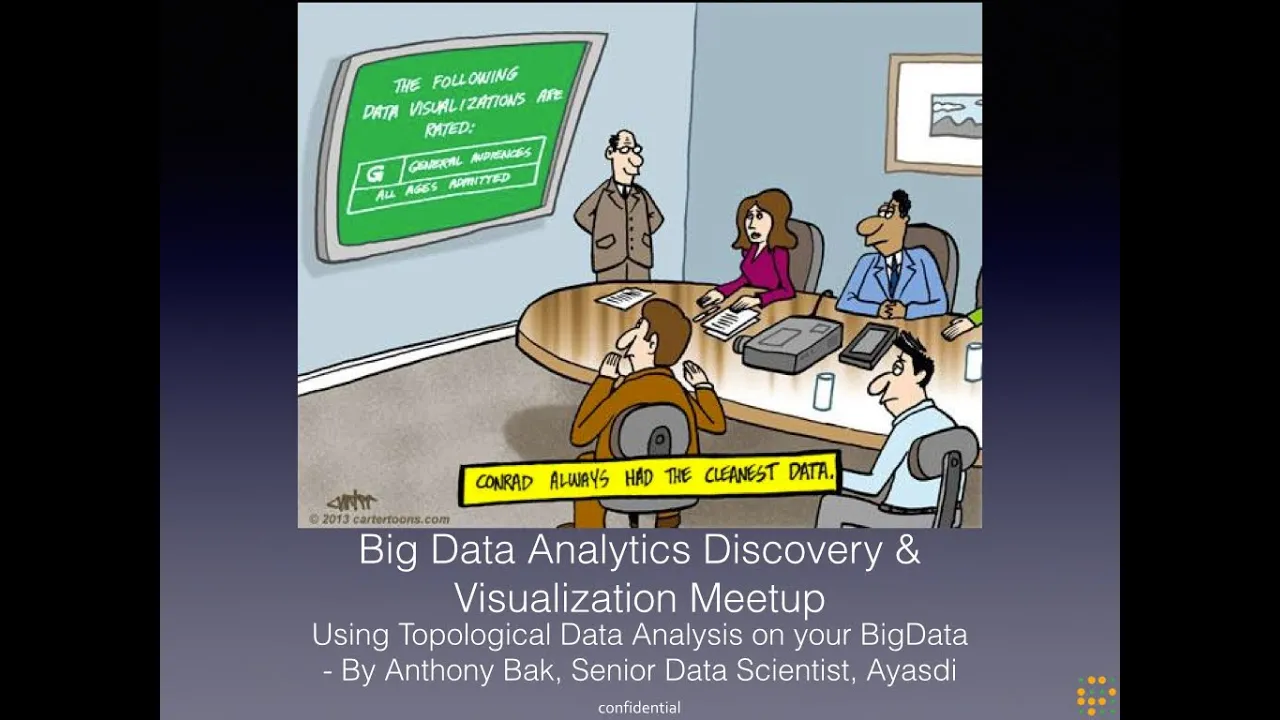
• Why this video is valuable: To round out your understanding of TDA, this video showcases its real-world value. It details how TDA can identify anomalies, fraud patterns, and structural features in noisy, high-dimensional datasets that traditional machine learning techniques often miss.

---

Computational Supplement: Python TDA Implementation

To supplement the limited video tutorials on modern libraries, use the following code block as a reference for setting up and running a persistent homology analysis using Ripser and Persim:

Setup your environment: pip install ripser persim numpy matplotlib

import numpy as np import matplotlib.pyplot as plt from ripser import ripser from persim import plot_diagrams

1. Generate a noisy circle (point cloud with a 1D hole)

np.random.seed(42) theta = np.random.uniform(0, 2*np.pi, 100) x = np.cos(theta) + np.random.normal(0, 0.05, 100) y = np.sin(theta) + np.random.normal(0, 0.05, 100) data = np.vstack((x, y)).T

2. Compute persistent homology (up to 1D loops)

dgms = ripser(data, maxdim=1)['dgms']

3. Plot the Persistence Diagram

H0 features (connected components) appear at birth=0.

The prominent H1 feature (the circular loop) will appear far from the diagonal.

plot_diagrams(dgms, show=True)

Knowledge Checkpoint

• How do you convert a persistence barcode interval $[b, d)$ into a coordinate point on a persistence diagram? What does a point close to the diagonal line represent?
• What is the bottleneck distance, and why is it important for proving that persistent homology is stable against noise?
• Can you run a Python script using ripser to compute and plot the persistence diagram of a noisy sphere?

---

Course Map

Below is the recommended path through the curriculum, showing how the modules build on each other from theoretical foundations to practical computation.

---

Key People Index

• Gunnar Carlsson (Stanford University): One of the pioneering mathematicians behind TDA. His work translated algebraic topology into computational algorithms, and he co-founded Ayasdi to apply TDA to industry problems.
• Henry Adams (University of Florida): A prominent educator and researcher in applied topology. His research and lecture series are excellent resources for learning persistent homology and its applications in machine learning.
• Elizabeth Munch (Michigan State University): A leading researcher in multidimensional persistence and TDA applications. Her tutorials and open-source contributions help bridge the gap between abstract math and practical data analysis.
• Francesca Tombari (KTH Royal Institute of Technology): An applied topologist known for her clear explanations of metric-space-associated simplicial complexes (Čech, Rips, Delaunay, and Alpha complexes).

---

Final Self-Assessment

Complete this self-assessment after finishing all five modules to verify your understanding of TDA:

• Topological Equivalence: I can intuitively explain continuous deformations and identify topological invariants.
• Algebraic Foundations: I understand how a vector space over a field works and can define the axioms of a group.
• Simplices: I can list the vertices and faces of an $n$-simplex and verify if a collection of simplices forms a valid simplicial complex.
• Complex Comparisons: I can explain why the Čech complex preserves homotopy while the Vietoris-Rips complex is computationally preferred.
• The Boundary Operator: I can apply the boundary operator $\partial_k$ to a simplex and algebraically prove that $\partial^2 = 0$.
• Homology Groups: I can define homology as the quotient group of cycles modulo boundaries ($H_k = Z_k / B_k$).
• Betti Numbers: I can calculate Betti numbers for basic shapes like a circle, torus, and sphere.
• Filtration: I can explain how a filtration is built by growing balls around data points and how this tracks features across scales.
• Matrix Reduction: I understand how to set up a boundary matrix and apply the column-reduction algorithm to find birth and death times.
• Visualizing Persistence: I can read and interpret both persistence barcodes and persistence diagrams, identifying which features represent structural signal.
• Stability: I can explain why the stability of persistent homology under bottleneck distance makes it useful for analyzing noisy real-world data.
• Practical Application: I can write a Python script using libraries like ripser or gudhi to compute the persistent homology of a custom point cloud dataset.