CMB (Lambda-CDM, Anisotropy & Polarization)
Learning Goal
Decipher the physics of the Cosmic Microwave Background (CMB) radiation, including its origin, the emergence of temperature anisotropies, the mechanics of linear polarization (E-modes and B-modes), and the methodology by which CMB observations constrain the six fundamental cosmological parameters of the standard model.
Prerequisites
To get the most out of this curriculum, you should be comfortable with:
- Introductory Physics: Basic thermodynamic concepts (blackbody radiation, thermal equilibrium) and electromagnetism (wave polarization, scattering).
- Mathematical Foundations: Familiarity with Fourier transforms, spherical harmonics, and statistical averages.
- Introductory Cosmology: Basic concepts of General Relativity (the metric of expanding space) and the FLRW metric are highly beneficial, though qualitative explanations are provided.
Estimated Total Study Time
18 Hours (includes video lectures, required reading, self-assessment, and mathematical deep-dives).
Module 1: Foundations of Cosmology & The Expanding Universe
This module builds the prerequisite physical framework of modern cosmology. You will explore how Einstein’s General Relativity shifted our paradigm from a static universe to a dynamic, stretching spacetime. You will master cosmic redshift (), Hubble's Law, and trace the thermal timeline of the early universe back to the hot, dense state of the early Big Bang.
Recommended Videos

Why this video
This video provides an elegant visualization of how Albert Einstein applied non-Euclidean geometry to physical space, showing that mass-energy curves spacetime. It helps you transition from the Newtonian worldview of absolute space to the relativistic understanding that spacetime is a dynamic entity capable of expanding, contracting, and warping—a fundamental prerequisite to understanding why the CMB is stretched and redshifted.
Why this video
Dr. Jason Kendall breaks down cosmic redshift () with mathematical clarity, distinguishing it from the standard Doppler effect. This video is essential for understanding how the stretching of space itself increases the wavelength of propagating photons, laying the exact foundation needed to calculate the temperature cooling of the CMB over cosmic time.
Why this video
Presented by Fermilab, this video bridges the gap between particle physics and early-universe cosmology. It outlines the thermal evolutionary timeline of the cosmos, illustrating how extreme temperatures in the first fractions of a second prevented the existence of bound atoms, keeping the universe in an ultra-dense, opaque plasma state.
Knowledge Checkpoint
- Explain the difference between kinematic Doppler redshift (motion through space) and cosmological redshift (expansion of space).
- Define redshift mathematically as a function of the scale factor : .
- Describe the thermodynamic relationship between the temperature of the universe and its scale factor , specifically proving why .
- Summarize the state of the universe during the radiation-dominated era and identify the primary particle interactions that maintained thermodynamic equilibrium.
Module 2: Origin and Discovery of the CMB
In this module, you will explore the transition of the universe from an opaque plasma to a transparent, neutral gas. You will study the physics of recombination and photon decoupling, understand how the CMB was serendipitously discovered, and analyze why the CMB remains the most mathematically perfect blackbody spectrum ever observed in nature.
Recommended Videos

Why this video
This highly detailed visual documentary walks through the transition of the early universe at . It explains how the cooling of the universe to allowed electrons to bind with protons to form neutral hydrogen, freeing photons from their continuous Thomson scattering off free electrons and initiating the "last scattering" event.

Why this video
This video explains the observational reality of the Last Scattering Surface (LSS). It visualizes the LSS as a spherical boundary surrounding us in all directions, representing the physical limit of our electromagnetic observations of the early universe.

Why this video
Part of Stanford University's graduate-level physics sequence, this lecture segment unpacks the quantitative mechanics of recombination. It explains the "recombination bottleneck" and uses the Saha Equation to demonstrate why recombination occurs at a much lower energy scale () than the actual ionization potential of ground-state hydrogen ().
Mathematical Deep-Dive: Recombination and Decoupling
To understand why decoupling occurs at () despite the ionization energy of hydrogen being , we look to the Saha Equation:
Because the ratio of photons to baryons (the baryon-to-photon ratio ) is incredibly small, there is an immense reservoir of high-energy photons in the Wien tail of the Planck distribution. Even at , these tail-end photons are numerous enough to immediately ionize neutral hydrogen. Recombination only stabilizes when the temperature drops low enough that the photon density above falls below the baryon density.
Knowledge Checkpoint
- Differentiate between recombination (electrons binding to protons) and decoupling (photons freeing themselves from Thomson scattering interactions).
- Explain why the CMB is an almost mathematically perfect blackbody spectrum, and list the thermalization processes (e.g., bremsstrahlung, double Compton scattering) that occurred prior to decoupling.
- Describe the historical significance of the Penzias and Wilson discovery at Bell Labs, explaining how they eliminated terrestrial noise to isolate the isotropic background hiss.
- Calculate the scale factor at the era of last scattering given that .
Module 3: CMB Temperature Anisotropies & The Power Spectrum
This module covers the physical origins of the tiny temperature fluctuations () imprinted on the last scattering surface. You will study Baryon Acoustic Oscillations (BAO), analyze the compete set of physical mechanisms driving anisotropies, and learn to dissect the angular power spectrum of the CMB.
Recommended Videos

Why this video
PBS Space Time delivers a highly intuitive explanation of Baryon Acoustic Oscillations. It explains the struggle between gravitational collapse (driven by dark matter and baryons) and outward radiation pressure (driven by photons), showing how this competition setup massive acoustic oscillations in the primordial plasma before they froze at decoupling.

Why this video
This segment visualizes the transition from a 2D temperature map of the sky to a 1D angular power spectrum. It illustrates how statistical correlation analysis extracts the power (amplitude of variance) at different angular scales, laying the visual groundwork for understanding multipole moments ().
Why this video
This video features working astrophysicists explaining how they calculate the correlations between sky regions to construct the CMB power spectrum. It helps demystify how the peaks and troughs in the power spectrum represent physical resonant scales in the early universe.
Pedagogical Deep-Dive: Deciphering the Angular Power Spectrum
To analyze the temperature fluctuations across the celestial sphere, astrophysicists expand the temperature field in terms of spherical harmonics:
The angular power spectrum is defined by the angular correlation coefficient , which averages the coefficients over all possible orientations ( modes):
Understanding the Multipole Index and Angular Scale
The multipole index corresponds inversely to an angular scale on the sky:
- Low (, ): Large angular scales. These scales were larger than the cosmic horizon at decoupling, meaning physical processes (like sound waves) had no time to affect them. They directly reflect the primordial quantum fluctuations seeded by inflation, modified by the Sachs-Wolfe effect (photons losing energy escaping gravitational potential wells).
- The First Acoustic Peak (, ): This peak represents the sound horizon at the moment of decoupling—the maximum distance a sound wave could travel since the beginning of the universe. It represents the fundamental mode of the acoustic oscillations (regions that underwent exactly one maximum compression before freezing).
- The Second Acoustic Peak (, ): This peak represents the first odd harmonic—regions that underwent exactly one maximum rarefaction (expansion) before freezing.
- The Third Acoustic Peak (, ): This represents the second compression peak.
Power [l(l+1)Cl / 2pi]
^
| |First Peak (l ~ 220)
| /
| / \ |Third Peak (l ~ 800)
| / \ |Second /
| / / Peak /
| / \ (l~540) \ /---\ Silk
|_/ _/ _/ _ Damping (l > 1000)
--------------------------------------------------------> Multipole Moment (l)
Low l (Large scales) High l (Small scales)
Knowledge Checkpoint
- State the relationship between the multipole index and the physical angular scale on the sky.
- Explain the physics behind the Sachs-Wolfe effect and explain why it dominates the angular power spectrum at very low multipoles ().
- Describe the physical mechanism driving the acoustic peaks: what forces act as the "spring" and what acts as the "mass" in these oscillations?
- What is Silk Damping (diffusion damping), and why does the power spectrum decay rapidly at very high multipole moments ()?
Module 4: CMB Polarization: E-modes and B-modes
This module explores the polarization of the CMB. You will study how unpolarized radiation becomes linearly polarized through Thomson scattering, the geometric classification of polarization patterns into gradient-like E-modes and curl-like B-modes, and how B-modes act as a detector for primordial gravitational waves from cosmic inflation.
Recommended Videos

Why this video
Dr. Matias Zaldarriaga, a pioneer in CMB polarization theory, explains the exact physical origin of polarization. He demonstrates how density fluctuations at the last scattering surface generate a local quadrupole anisotropy in the radiation field, which is required to produce net linear polarization via Thomson scattering.
Why this video
This lecture provides the mathematical definition of polarization using Stokes parameters ( and ). It details how these coordinate-dependent parameters are transformed into the coordinate-independent scalar fields of E-modes (curl-free) and B-modes (curl-like).

Why this video
This video explains the experimental hunt for primordial B-mode polarization using ground-based telescopes like BICEP. It details why detecting B-modes is considered the "smoking gun" for the theory of cosmic inflation, while also explaining the challenge of distinguishing cosmic signals from galactic dust foregrounds.
Pedagogical Deep-Dive: Thomson Scattering & Polarization Mechanics
Linear polarization of CMB photons is generated at the LSS only when a free electron scatters radiation that has a local quadrupole anisotropy (meaning the electron is illuminated by hotter radiation from one orthogonal direction and colder radiation from the other).
     Hot Photon (y-axis)
          |
          | (High Intensity)
          v
Unpolarized --(Electron)-- Unpolarized Light (x) ^ | (Low Intensity) | Cold Photon
When the unpolarized radiation fields along the x and y axes scatter off the electron, the transverse nature of electromagnetic waves ensures that the scattered wave propagating along the z-axis (out of the page) retains a net linear polarization.
E-modes vs. B-modes
The polarization field on the sky is a tensor field characterized by Stokes parameters and . To remove coordinate system dependence, we decompose this tensor field into two distinct scalar modes:
-
E-modes (Gradient-like): These are symmetric under parity reflection (parity-even). Their polarization vectors are either parallel or perpendicular to the direction of the temperature gradient. They are generated by scalar density perturbations (acoustic waves).
-
B-modes (Curl-like): These are anti-symmetric under parity reflection (parity-odd). Their polarization vectors are oriented at angles relative to gradients, displaying a clear spiral/handedness pattern. They cannot be generated by scalar density perturbations at linear order. They are generated only by tensor perturbations (gravitational waves stretching spacetime itself) or by the gravitational lensing of E-modes as they travel to us.
E-Mode (Curl-Free) B-Mode (Curl-Like)
    |   |                               \   \
  --+---+--                               \   \
    |   |                               /   /
  --+---+--                               /   /
Video Gap Acknowledgment & Self-Study Advice
Note on Video Resources: While the video pool contains high-level research lectures, there is a relative lack of intuitive 3D animated tutorials showing the precise projection of Stokes and parameters onto sphere coordinates.
To supplement this module, we highly recommend searching YouTube independently for:
- "CMB Polarization E-modes and B-modes animation"
- "Wayne Hu CMB polarization tutorial"
- Reading suggestion: Read Wayne Hu's online tutorial pages on "CMB Polarization" for a comprehensive step-by-step mathematical guide.
Knowledge Checkpoint
- Explain why a monopole or dipole radiation field incident on a free electron produces zero net linear polarization after scattering.
- Define the Stokes parameters and and describe how they behave under a coordinate rotation.
- Highlight the structural difference between E-modes and B-modes in terms of their parity transformations.
- Explain how gravitational lensing acts as a foreground contaminant by converting E-mode polarization into B-mode polarization on small angular scales.
Module 5: Constraining the Lambda-CDM Cosmological Parameters
In this final module, you will learn how the position, height, and relative ratios of the CMB temperature and polarization peaks are used as high-precision cosmic scales. You will discover how the Planck satellite data is used to constrain the six fundamental parameters of the standard model of cosmology.
Recommended Videos

Why this video
This comprehensive academic presentation from Harvard's Radcliffe Institute explains how the standard model of cosmology () is constructed. It details how the first three acoustic peaks of the CMB power spectrum constrain spatial curvature, baryon density, and dark matter density.

Why this video
Laura Herold presents a clear breakdown of how the CMB constrains the Hubble constant () through the angular scale of the sound horizon (). The talk provides a critical transition into modern debates, explaining the "Hubble Tension" between CMB-derived values and local distance ladder measurements.
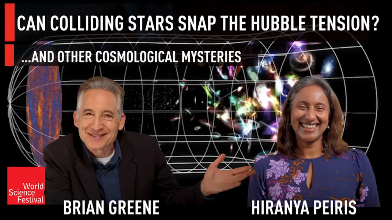
Why this video
This panel discussion from the World Science Festival outlines the physical components of the model. It discusses the current crisis in cosmology surrounding the discrepancy in expansion rate measurements, helping you understand how robust the CMB constraints are compared to alternative models.
How the Peaks Constrain the 6 Parameters
The standard model is fully defined by six fundamental parameters. We constrain them using specific physical characteristics of the CMB power spectrum:
| Parameter | Symbol | Physical Mechanism of CMB Constraint |
|---|---|---|
| Baryon Density | Baryon Loading: Adding baryons increases the mass of the plasma "fluid," dragging down the rarefaction peaks. A higher baryon density increases the height of the first and third peaks relative to the second peak. | |
| Cold Dark Matter Density | Matter-Radiation Equality: Dark matter provides gravitational potential wells without outward pressure. A higher dark matter density reduces the radiation-driving effect, changing the overall amplitude of the third peak relative to the first peak. | |
| Angular Sound Horizon | Geometric Ruler: This determines the precise angular position (-position) of the first acoustic peak. Because the physical size of the sound horizon is known, its angular projection on the sky acts as a standard ruler, determining the spatial curvature () of the universe. | |
| Optical Depth to Reionization | Scattering Suppression: When the first stars lit up and reionized the universe, free electrons scattered CMB photons. This dampens the temperature power spectrum fluctuations by a factor of at high . | |
| Primordial Amplitude | Overall Normalization: This parameter scales the overall height of the entire power spectrum, representing the starting power of primordial quantum fluctuations. | |
| Scalar Spectral Index | Tilt of the Spectrum: This measures how the amplitude of primordial fluctuations varies with scale. A value of is scale-invariant; (red tilt) means larger physical scales have slightly higher amplitude fluctuations than smaller scales, changing the slope of the power spectrum baseline. |
Knowledge Checkpoint
- Explain how "baryon loading" affects the relative heights of the odd (compression) and even (rarefaction) peaks in the CMB power spectrum.
- Detail how the precise angular position of the first acoustic peak () proves that our universe is spatially flat ().
- What is the "Hubble Tension"? Contrast how the CMB measures indirectly via the sound horizon versus how the distance ladder measures it directly using Cepheid variables and Supernovae.
- Why does cosmic reionization at suppress the CMB temperature fluctuations at high multipoles?
Course Map
Key People Index
- Albert Einstein: Formulated General Relativity (1915), providing the geometric spacetime framework that allows for cosmic expansion.
- Edwin Hubble: Discovered cosmic expansion (1929) by establishing a linear relationship between galactic redshift and distance.
- Arno Penzias & Robert Wilson: Serendipitously discovered the CMB radiation (1964) using the Holmdel Horn Antenna at Bell Labs, earning the 1978 Nobel Prize in Physics.
- George Gamow, Ralph Alpher, & Robert Herman: Predicted the existence of a cosmic relic radiation field (CMB) in 1948 based on early universe nucleosynthesis calculations.
- Matias Zaldarriaga & Usel Seljak: Developed the theoretical formalism for decomposing CMB polarization into E-modes and B-modes (1997), and created the widely used CMBFAST software.
- Alan Guth: Proposed the theory of cosmic inflation (1981), which provides the physical mechanism for producing the flat spatial geometry and primordial scalar and tensor perturbations.
Final Self-Assessment
Complete this comprehensive self-assessment to verify your mastery of the curriculum:
- I can calculate the cosmological redshift given emitted and observed wavelengths, and relate it directly to scale factor .
- I can explain the physical difference between the epoch of recombination and the epoch of photon decoupling.
- I can explain why the CMB spectrum deviates by less than from a perfect blackbody spectrum.
- I can mathematically relate a multipole index to its corresponding angular scale on the sky.
- I can describe the three main physical mechanisms of temperature anisotropies: gravity (Sachs-Wolfe), density/temperature variations (intrinsic), and velocity (Doppler).
- I can explain why baryon loading suppresses the second acoustic peak while enhancing the first and third peaks.
- I can explain why a quadrupole anisotropy is required to generate linear polarization through Thomson scattering.
- I can draw or describe E-mode (parity-even) and B-mode (parity-odd) polarization patterns on a flat plane.
- I can list the six primary parameters of the standard model and describe which features of the CMB power spectrum constrain each of them.
- I can explain the origin of primordial B-modes (inflationary gravitational waves) and contrast them with late-time lensed B-modes.