Mapping Dark Matter: Gravitational Lensing
Learning Goal: Analyzing the physics of strong and weak gravitational lensing to map the distribution of dark matter in galaxy clusters and individual galaxies.
- Prerequisites: Multivariable calculus, introductory classical mechanics (Newtonian gravity), and basic electromagnetism (wave propagation).
- Estimated Total Study Time: 20 Hours
Module 1: Foundations of General Relativity and Spacetime
Overview
To understand why light bends across the universe, we must abandon the Newtonian concept of gravity as an instantaneous, straight-line force. This module introduces Albert Einstein's General Theory of Relativity, focusing on how mass and energy warp the four-dimensional fabric of spacetime, forcing light paths to follow curved trajectories called null geodesics.
Recommended Videos

Why this video
Delivered by theoretical physicist Leonard Susskind, this classic Stanford lecture uses the equivalence principle to show why gravity bends light. By comparing a stationary frame in a gravitational field to an accelerating elevator, Susskind walks through the kinematic derivation of light bending, showing that the path of a horizontal light ray must curve downward in an accelerating frame.
Why this video
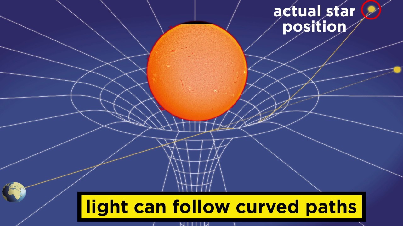
This video provides an intuitive visual transition from Newton's gravitational model to Einstein's geometric model. It explains how massive bodies deform spacetime coordinates, visually demonstrating why objects (including photons) traveling in straight paths actually follow curved paths (geodesics) through warped space.
Why this video
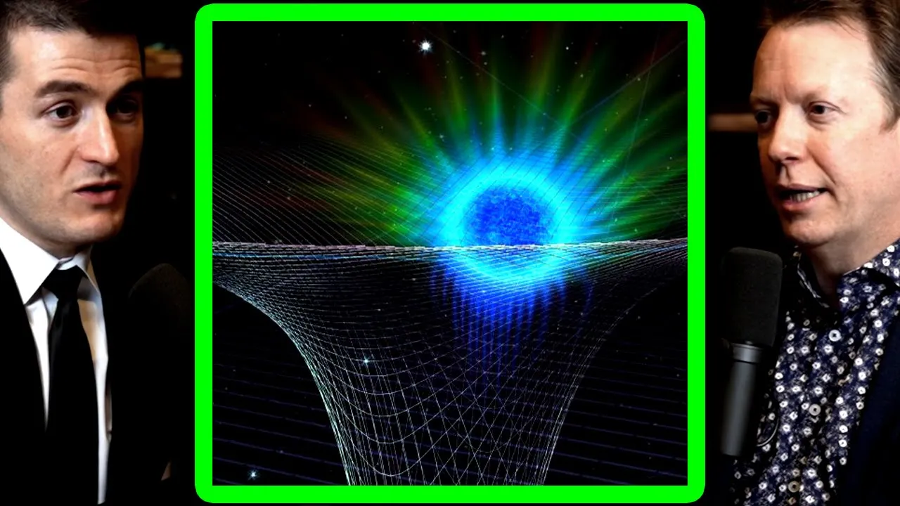
In this conversational yet deep explanation, theoretical physicist Sean Carroll explains the core concept of General Relativity: matter tells spacetime how to curve, and spacetime tells matter how to move. This video provides a conceptual bridge between the mathematics of the metric tensor and observable astrophysical phenomena.
Knowledge Checkpoint
- Understand the Equivalence Principle and how it demands the bending of light in a gravitational field.
- Define a "geodesic" and explain why light follows curved paths despite having zero rest mass.
- Explain how Einstein's field equations relate spacetime curvature to mass-energy density.
Module 2: Cosmology and the Evidence for Dark Matter
Overview
This module establishes the cosmological context of dark matter. Students will explore observational anomalies—primarily galactic rotation curves and galaxy cluster velocities—that cannot be explained by visible matter, showing why dark matter is an essential pillar of our standard model of cosmology (CDM).
Recommended Videos

Why this video
This comprehensive, academically rigorous video explains why dark matter is treated as an observed physical phenomenon rather than a loose hypothesis. It details the history of galaxy rotation curves, the contributions of Vera Rubin and Fritz Zwicky, and how alternative theories like MOND (Modified Newtonian Dynamics) struggle to explain the broader range of observations that dark matter easily accounts for.

Why this video
This lecture focuses on the mathematical derivation of galactic rotation curves. It shows how Newtonian dynamics predicts that outer stellar orbital speeds should fall off as based on visible mass distributions, and contrasts this prediction with the observed flat rotation curves (), proving the existence of a massive, invisible dark matter halo.

Why this video
This video profiles Fritz Zwicky’s 1933 discovery of mass discrepancies in the Coma Cluster and Vera Rubin’s subsequent work on spiral galaxies. It serves as an excellent introduction to why baryonic (normal) matter is insufficient to bind large-scale structures, setting the stage for gravitational lensing as the ultimate mapping tool.
Knowledge Checkpoint
- Derive the expected Newtonian rotation velocity for stars outside a galaxy's optical radius and explain the flat curves observed in real data.
- Explain how Fritz Zwicky used the Virial Theorem to conclude that the Coma Cluster contains far more mass than is visible.
- Summarize the primary components of the CDM model and the estimated percentages of dark matter, dark energy, and baryonic matter.
Module 3: Physics of Strong Gravitational Lensing
Overview
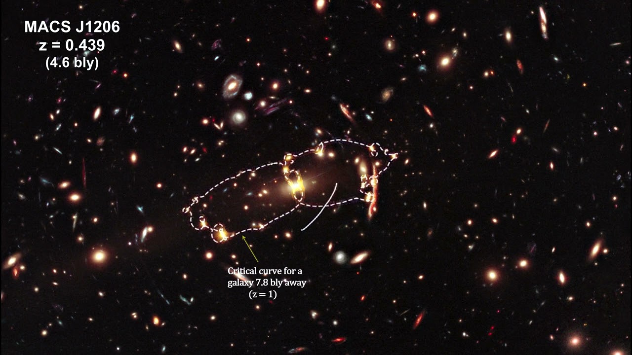
When a massive object (like a galaxy or cluster) aligns closely with a background light source, it acts as a cosmic lens. This module covers the core geometric optics of strong gravitational lensing, the derivation of the lens equation, the Einstein radius, and the formation of highly distorted images, including Einstein rings, arcs, and multiple images.
Recommended Videos

Why this video
This video explains the thin-lens approximation and the fundamental lens equation, which relates the observed image position () to the true source position () through the deflection angle (). It offers a great, concise mathematical visualization of the geometric configuration of the observer, lens, and source planes.
Why this video
This video offers clean 3D animations and astronomical observations of Einstein rings and gravitational arcs. It illustrates how perfect alignment yields rings, while small offsets produce multiple discrete images or stretched arcs.
Why this video
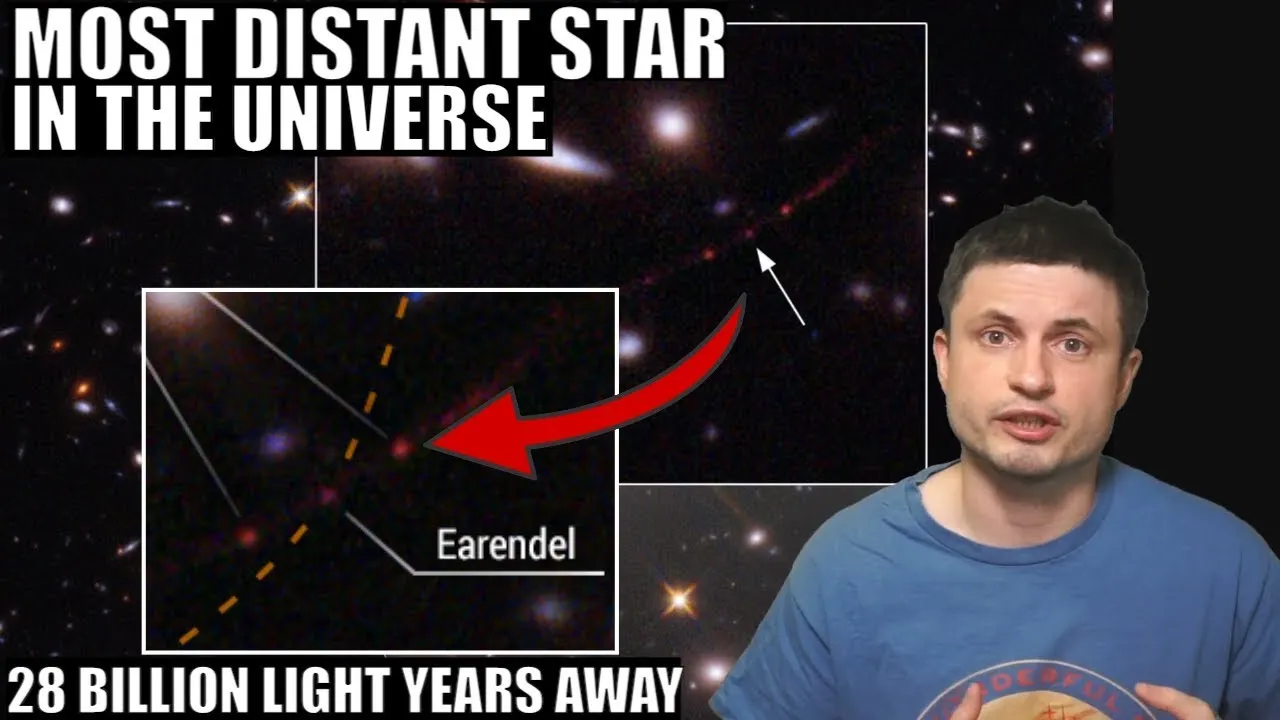
This video presents a real-world case study of strong lensing: the discovery of Earendel, a star magnified thousands of times by an intervening galaxy cluster. It illustrates "critical curves" and "caustics"—boundaries in the source and lens planes where magnification theoretically diverges to infinity.
Supplemental Mathematics: Derivation of the Lens Equation
Curriculum Gap Note: Existing video content focuses on qualitative explanations of strong lensing. To master this topic, work through the following mathematical derivation:
    Source (S)
      o  [True Position: beta]
     / \
    /   \
   /     \  Deflection Angle (alpha)
  /       \
 /       (L) Lens (Mass M)
/         |
/ | [Observed Position: theta] / | o------------+--------------------o Observer (O) <- - - D_L - ->[Lens Plane] < - - - - - - D_S - - - - - - - - >[Source Plane]
- Light Deflection Angle (): For a point mass with an impact parameter (where ), General Relativity predicts a deflection angle of:
- The Lens Equation (Thin Lens Approximation): Using the geometry of the diagram above, the relationship between the true source angular position and the observed angular position is: where the scaled deflection angle is: Therefore:
- The Einstein Radius (): When the source is perfectly aligned behind the lens (), the lensed image forms a symmetric ring. Solving for under this condition yields the Einstein Radius:
Knowledge Checkpoint
- Derive the lens equation from the geometric relationship between the observer, lens, and source planes.
- Calculate the Einstein radius (in arcseconds) for a galaxy of mass acting as a lens at with a source at .
- Explain how multiple images are produced by solving the lens equation for non-zero source offsets ().
Module 4: Physics of Weak Gravitational Lensing
Overview
Unlike strong lensing, which requires near-perfect alignment and produces dramatic arcs, weak gravitational lensing is a statistical phenomenon. It slightly distorts the shapes of almost all background galaxies. This module introduces the mathematical framework of weak lensing, detailing how the gravitational potential field creates shear (stretching) and convergence (magnification) across the sky.
Recommended Videos

Why this video
This academic lecture explains the physics of the weak lensing regime. It demonstrates how an individual galaxy's light is slightly distorted when passing through a mass distribution, showing how astronomers use statistical averages of multiple background galaxies to reconstruct the shape profile of a lens.

Why this video
This lecture provides the mathematical foundation of cosmic shear. Alonso presents the key observational equation: the observed ellipticity () is the sum of the true unlensed ellipticity () and the gravitational shear (). Since galaxy orientations are randomly distributed, averaging over many galaxies allows astronomers to isolate the shear term.

Why this video
This long-form, highly advanced academic lecture goes deep into the observational challenges of weak lensing. Bernstein explains how systematic errors, telescope optics (Point Spread Function), and detector noise distort galaxy shapes, and discusses the statistical correction methods required to extract clean lensing signals.
Supplemental Mathematics: Shear vs. Convergence
Curriculum Gap Note: To bridge the gap between qualitative overviews and Bernstein's highly advanced lecture, study this mathematical breakdown of the Jacobian matrix mapping background sources to observed images.
The distortion of an image is described by the Jacobian matrix , which maps coordinates in the source plane to coordinates in the image plane:
This matrix is decomposed into two main physical components:
-
Convergence ():
- Definition: A scalar field representing the isotropic magnification of the source (changes size and flux, but preserves shape).
- Physics: Proportional to the projected local surface mass density divided by the critical surface mass density :
-
Shear ():
-
Definition: A complex trace-free tensor describing anisotropic stretching (stretches circular sources into ellipses).
-
Physics: Directly related to the tidal gravitational forces of the lens. represents stretching along the x/y axes, while represents stretching at angles.
Unlensed Convergence (kappa) Shear (gamma) [O] ( O ) ( O ) Circular Source Isotropic expansion Anisotropic stretching
-
Knowledge Checkpoint
- Write down the deformation matrix and explain the geometric impact of convergence () versus shear ().
- Explain why the average unlensed ellipticity of a large population of galaxies is assumed to be zero.
- Explain how the Point Spread Function (PSF) of a telescope can mimic weak lensing shear, and describe one method used to correct for it.
Module 5: Dark Matter Mass Reconstruction and Mapping
Overview
This capstone module synthesizes strong and weak lensing data into a unified framework for mapping dark matter. Students will learn the step-by-step pipeline used by cosmologists to convert observed galaxy ellipticities into 2D and 3D density maps of galaxy clusters, with a focus on computational modeling using software like lenstronomy and Lenstool.
Recommended Videos
Why this video
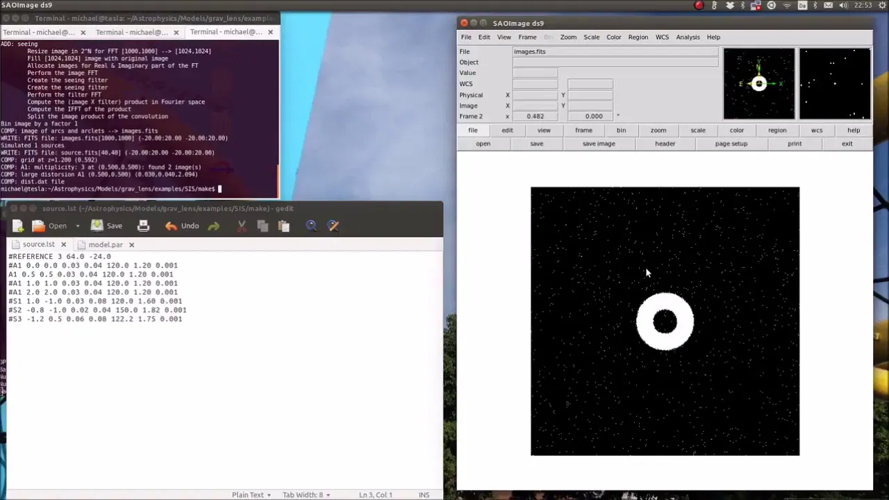
This computational walkthrough shows how researchers reconstruct mass distributions in practice. The tutorial demonstrates how to use the open-source software Lenstool to model galaxy-galaxy lensing using Singular Isothermal Sphere (SIS) and Ellipsoid (SIE) mass profiles, showing how observational data is fitted to physical parameters.
Why this video
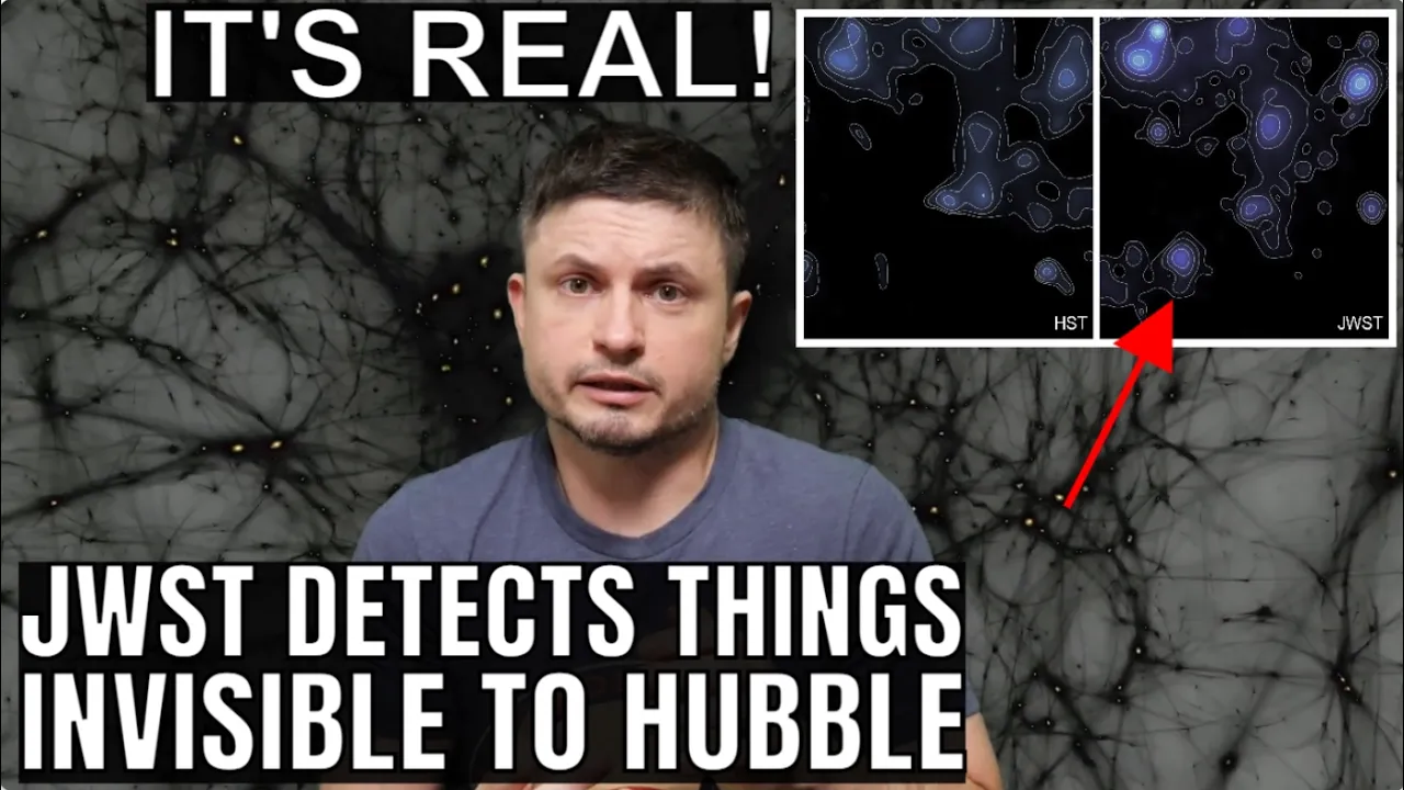
Using recent James Webb Space Telescope data, this video explains how weak lensing measurements of minor 1% distortions are combined over millions of background galaxies to reconstruct the "cosmic web" of dark matter filaments.

Why this video
Though brief, this clip displays the overlay mapping of the Bullet Cluster (1E 0657-568). It shows the critical offset between baryonic matter (hot gas seen in pink by Chandra X-ray) and total mass (mapped in blue by weak lensing), which serves as direct proof of dark matter.
Computational Pipeline: Mass Mapping Walkthrough
Curriculum Gap Note: To address the lack of technical walkthroughs for lensing reconstruction, review this Python/
lenstronomypipeline overview.
To map dark matter, astronomers must invert the observed shear field to find the underlying mass density field (convergence ). This is done using the Kaiser-Squires Inversion algorithm:
[Background Galaxies] ---> Measure Ellipticities (e_obs) ---> Grid & Average to create Shear Field (gamma_1, gamma_2) | [Dark Matter Map] <--- Project Convergence (kappa) <--- Kaiser-Squires Inversion (Fourier Domain)
Step-by-Step Computational Workflow:
- Catalog Generation: Collect shapes, positions, and estimated redshifts of background galaxies.
- PSF Correction: Deconvolve the telescope's point spread function from the galaxy image shapes to extract the pure gravitational shear.
- Fourier Transformation: In the Fourier domain, shear () and convergence () are related by a simple algebraic projection. First, transform the real-space shear fields:
- Kernel Application (Inversion): Compute the convergence in Fourier space:
- Inverse Fourier Transform: Transform back to real space to yield the mass density map:
- Visualization: Plot the 2D convergence map to reveal dark matter overdensities.
Knowledge Checkpoint
- Explain the steps of the Kaiser-Squires inversion algorithm and how it extracts the convergence field from shear measurements.
- Describe the physical significance of the Bullet Cluster separation and why MOND struggles to explain this observation.
- Set up a basic lensing model using
Lenstoolor Python'slenstronomypackage, specifying the lens mass profile (e.g., SIS or NFW) and the source profile.
Course Map
Key People Index
| Researcher | Primary Context / Contribution | Mentioned in Module(s) |
|---|---|---|
| Albert Einstein | Formulated General Relativity, predicted gravitational light bending and the lens equation. | Modules 1, 3 |
| Arthur Eddington | Led the 1919 solar eclipse expedition that confirmed the gravitational deflection of light by the Sun. | Module 1 |
| Fritz Zwicky | First proposed "dark matter" (dunkle Materie) in 1933 after observing mass anomalies in the Coma cluster. | Module 2 |
| Vera Rubin | Provided observational proof of dark matter halos through spiral galaxy rotation curves. | Module 2 |
| Gary Bernstein | Pioneer in weak gravitational lensing measurements and PSF correction methodologies. | Module 4 |
| Nick Kaiser &<br>Gerard Squires | Developed the Kaiser-Squires inversion algorithm, creating the mathematical foundation for dark matter mass mapping. | Module 5 |
Final Self-Assessment
Complete this comprehensive self-assessment to verify your mastery of the physics of gravitational lensing and dark matter mapping.
- Equivalence Principle: I can explain how Einstein used an accelerating elevator thought experiment to predict that gravity bends light.
- Geodesic Trajectory: I can mathematically define a null geodesic and explain why photons travel along them in curved spacetime.
- Rotation Curves: I can derive the flat velocity curve relationship using a dark matter halo mass profile () and contrast it with the Keplerian fall-off ().
- Lens Geometry: I can derive the lens equation from a diagram of the observer, lens, and source planes.
- Einstein Radius: I can calculate the angular radius of an Einstein Ring given the mass of a lens and the angular diameter distances , , and .
- Shear vs. Convergence: I can explain the physical and geometric difference between isotropic convergence () and complex shear ().
- Jacobian Transformation: I can write out the magnification matrix and compute the magnification factor in terms of and .
- Kaiser-Squires Inversion: I can explain how the Kaiser-Squires algorithm operates in the Fourier domain to reconstruct convergence fields from measured shear.
- Bullet Cluster Physics: I can explain how the spatial offset between hot gas (X-ray emission) and total mass (weak lensing reconstruction) serves as empirical proof of dark matter.
- Modeling Frameworks: I can describe the setup, input data, and basic parameters required to run a mass reconstruction model in computational tools like
lenstronomyorLenstool.