Finding Exoplanets: Detection & Spectroscopy

Learning Goal: Mastering the detection methods and atmospheric analysis techniques used by modern astronomers to discover and characterize potentially habitable exoplanets.

Welcome to this rigorous, self-paced curriculum designed to take you from the foundational physics of astrophysics to the cutting edge of astrobiology and optical instrumentation. By navigating these 5 modules, you will transition from qualitative wonder to quantitative understanding of how humanity finds and analyzes worlds orbiting other stars.

• Prerequisites: Basic high school algebra and physics (familiarity with wave mechanics and Newton's laws of motion).
• Estimated Study Time: 15 hours.

Module 1: Foundations of Planetary Astrophysics

To characterize worlds light-years away, we must first master the language of light and gravity. This module establishes the physical baselines: how light behaves across the electromagnetic spectrum, how stars function (and how we measure their fundamental parameters), and the laws of orbital mechanics that govern planetary motion.

Recommended Videos

Light: Crash Course Astronomy #24

@crashcourse10:342751319

Light: Crash Course Astronomy #24

Light is a form of electromagnetic radiation whose wavelength determines its energy and color; shorter wavelengths correspond to higher energy (bluer light) and longer wavelengths to lower energy (redder light). Astronomers use spectroscopy to analyze the light emitted by celestial objects, which reveals their temperature, density, motion, spin, and chemical composition. Different atoms emit or absorb light at specific wavelengths, creating unique spectral fingerprints that allow scientists to i

@crashcourse · 10:34

• Why this video: Understanding light is the single most important prerequisite for astronomical detection. This video introduces the electromagnetic spectrum, wave-particle duality, and how atomic absorption/emission lines provide "fingerprints" of chemical components—concepts central to both radial velocity measurements and transit spectroscopy.

Basic Stellar Properties--the HR Diagram

@matthewmalkan13740:281420

Basic Stellar Properties--the HR Diagram

Astronomers measure two fundamental stellar properties—surface temperature (from spectral analysis of absorption lines) and luminosity (intrinsic power output)—to understand how stars work; stellar parallax measures distances by detecting the apparent wobble of nearby stars against distant background stars as Earth orbits the Sun, enabling calculation of luminosity via the inverse square law; plotting these properties on the Hertzsprung-Russell diagram reveals that over 90% of stars lie on the m

@matthewmalkan137 · 40:28

• Why this video: We cannot characterize a planet without first understanding its host star. This academic lecture dives deeply into stellar classification, surface temperatures, and absolute luminosity using the Hertzsprung-Russell (H-R) diagram, establishing how astronomers calculate stellar masses and radii.

What are Kepler's Laws of Planetary Motion? \| Orbits of Planets \| The Dr Binocs Show \| Peekaboo Kidz

@Peekaboo_Kidz6:25404851

What are Kepler's Laws of Planetary Motion? \| Orbits of Planets \| The Dr Binocs Show \| Peekaboo Kidz

Kepler's three laws describe how planets orbit the Sun: (1) Planets follow elliptical orbits with the Sun at one focus; (2) A line from the Sun to a planet sweeps equal areas in equal time intervals; (3) The square of a planet's orbital period is proportional to the cube of its semi-major axis. These laws, discovered by German astronomer Johannes Kepler in the early 17th century, explain the fundamental patterns governing planetary motion throughout our solar system.

@Peekaboo_Kidz · 6:25

• Why this video: Kepler's Laws form the bedrock of orbital mechanics. While designed as a basic conceptual visualizer, this video details how elliptical paths, equal orbital areas over equal times, and orbital periods dictate the mechanics of any planetary system.

Coverage Gaps & Independent Study

⚠️ Curriculum Note on Kepler's Laws: While the provided video is a fantastic visual introduction, it lacks the mathematical depth required to apply these laws analytically.

To master this mathematically, you must be able to work with Newton's derivation of Kepler's Third Law:

$P^2 = \frac{4\pi^2 a^3}{G(M_* + M_p)}$

Where $P$ is the orbital period, $a$ is the semi-major axis, $G$ is the gravitational constant, $M_*$ is the stellar mass, and $M_p$ is the planetary mass.

• Recommended independent search query: "Kepler's laws mathematical derivation lecture" or "Derivation of Kepler's Third Law Newtonian mechanics".

Knowledge Checkpoint

• Can you define the relationship between wavelength, frequency, and photon energy ($E = h\nu = \frac{hc}{\lambda}$)?
• Do you understand how an absorption line is formed in a stellar atmosphere?
• Can you locate where our Sun lies on the H-R diagram and explain how stellar mass correlates with main sequence lifetime?
• Can you state Kepler's three laws and explain how orbital speed varies from periastron to apastron?

Module 2: Exoplanet Detection Techniques

This module covers the primary techniques used to discover exoplanets: transit photometry and radial velocity (Doppler spectroscopy). We transition from qualitative conceptual graphics to the mathematical mechanics of orbital tugs and transit depths.

Recommended Videos

ExoDet2A: The RV Equation \| 2. Radial Velocities \| EXOPLANET DETECTION

@CoolWorldsClassroom11:413283

ExoDet2A: The RV Equation \| 2. Radial Velocities \| EXOPLANET DETECTION

The radial velocity method detects exoplanets by measuring the Doppler shift of a star's light, revealing reflex motion caused by gravitational tugging from orbiting planets; the resulting RV signal amplitude (K) depends on the planet's mass, orbital period, stellar mass, and orbital inclination, with the formula K = (2πG^(1/3)M_p^(2/3))/(P^(1/3)(M_*)^(1/3)) × sin(I), where the sin(I) term means RV measurements only provide minimum planet masses rather than true masses.

@CoolWorldsClassroom · 11:41

• Why this video: This video bridges the qualitative-quantitative gap by deriving the actual radial velocity (RV) semi-amplitude equation. It demonstrates how a planet's mass ($M_p$), orbital period ($P$), and inclination ($i$) determine the observable movement of its host star.

8.01x - Lect 23 - Doppler Effect, Binary Stars, Neutron Stars & Black Holes

@lecturesbywalterlewin.they92591:17134498

8.01x - Lect 23 - Doppler Effect, Binary Stars, Neutron Stars & Black Holes

By measuring the Doppler shift of absorption lines in a star's spectrum, astronomers can determine the star's radial velocity (motion toward or away from us). The formula λ'/λ = 1 + v/c × cosθ allows calculation of velocity. For example, if λ'/λ = 1.00333, the velocity is approximately -100 km/s (negative indicates recession). This only measures the radial component, not the full 3D velocity.

@lecturesbywalterlewin.they9259 · 1:17

• Why this video: An academic lecture from MIT detailing the pure physics of the Doppler effect. This provides the mathematical framework for how light waves shift based on velocity:

  $\frac{\Delta \lambda}{\lambda_0} \approx \frac{v_r}{c}$

  This fundamental equation is the mechanism behind Doppler spectroscopy.

Exoplanets: The Quest for Strange New Worlds (live public talk)

@NASAJPL1:04221972

Exoplanets: The Quest for Strange New Worlds (live public talk)

The Doppler spectroscopy method detects planets by measuring tiny velocity changes in a star's spectrum as it moves toward and away from us due to planetary gravitational tugging. Jupiter produces a ~12 m/s signal over 12 years; Earth-like planets produce ~10 cm/s signals. Hundreds of planets have been discovered using this technique.

@NASAJPL · 1:04

• Why this video: A comprehensive, high-level lecture delivered by JPL scientists that frames these mathematical detection techniques within the history of actual mission operations. It highlights real historical discoveries, instrumental challenges, and the complementary nature of transit and RV data.

Coverage Gaps & Independent Study

⚠️ Curriculum Note on Transit Mathematics: The pool lacks a rigorous step-by-step mathematical breakdown of transit light curves.

To quantitatively evaluate transit events, you must know how to calculate the transit depth ($\delta$), which is directly related to the ratio of the planet's cross-sectional area to the star's:

$\delta = \left(\frac{R_p}{R_*}\right)^2$

• Recommended independent search query: "Exoplanet transit depth calculation equation tutorial" and "Radial velocity method exoplanet mathematics derivation lecture".

Knowledge Checkpoint

• Can you derive the mass of an exoplanet ($M_p \sin i$) using the radial velocity semi-amplitude equation when stellar mass ($M_*$) and orbital period ($P$) are known?
• Why does the radial velocity method only give us a lower limit of the planet's mass ($M \sin i$), and how does a transit observation resolve this inclination ambiguity?
• If a star has a radius of $1 R_\odot$ and its transit signal shows a depth of $1\%$, what is the radius of the transiting exoplanet in terms of Jupiter radii ($R_J \approx 0.1 R_\odot$)?
• Explain how the tilt/inclination of an exoplanetary system affects our ability to detect it using both the transit and RV methods.

Module 3: Atmospheric Characterization & Spectroscopy

Once an exoplanet is detected, the next scientific frontier is figuring out what it is made of. This module covers exoplanet atmospheres using transmission and emission spectroscopy, focusing on the latest chemical data retrieved by the James Webb Space Telescope (JWST).

Recommended Videos

JWST discovered PHOTOCHEMISTRY in an exoplanet's atmosphere (this is a BIG deal) ft. Dr. Jake Taylor

@DrBecky11:34803632

JWST discovered PHOTOCHEMISTRY in an exoplanet's atmosphere (this is a BIG deal) ft. Dr. Jake Taylor

The James Webb Space Telescope's Early Release Science Program served as a proof-of-concept initiative to demonstrate JWST's capabilities across different scientific fields. Wasp 39b was specifically selected for observation due to several advantageous characteristics: strong water vapor absorption features detectable with Spitzer, an extremely short orbital period of only 4 Earth days enabling frequent observation opportunities, low density creating large extended atmospheres producing strong s

@DrBecky · 11:34

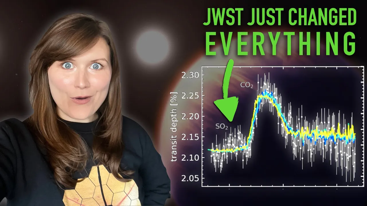
• Why this video: An elite-tier explanation of exoplanet photochemistry. It walks through how JWST observed WASP-39b to detect sulfur dioxide ($SO_2$) for the first time, explaining the chemical reaction pathways triggered by high-energy stellar photons hitting atmospheric compounds.

JWST has taken the most DETAILED spectrum of an exoplanet EVER

@DrBecky10:31281744

JWST has taken the most DETAILED spectrum of an exoplanet EVER

The James Webb Space Telescope has captured the most detailed spectrum of an exoplanet ever taken, revealing silicates (sand-like particles) in the atmosphere of VHS 1256b, a massive object orbiting two stars that sits on the boundary between planets and brown dwarfs; this spectrum also shows variability caused by dusty clouds and storms, and will help scientists determine whether VHS 1256b is a planet or a failed star by searching for deuterium fusion signatures.

@DrBecky · 10:31

• Why this video: This video breaks down how to read and interpret a raw atmospheric spectrum. It focuses on the discovery of silicate clouds in the atmosphere of VHS 1256b, teaching you how specific absorption and scattering features translate to physical climate states on other worlds.

Exoplanet Atmospheres

@degreesofscience8:54665

Exoplanet Atmospheres

Scientists analyze exoplanet atmospheres by observing starlight that filters through the planet's atmosphere during transit, where different molecules like water, methane, and carbon dioxide absorb light at specific wavelengths, allowing researchers to determine atmospheric composition; the James Webb Space Telescope enables this analysis for planets tens of light years away, with the first rocky planet confirmed by JWST being Earth-like in composition but orbiting a smaller red dwarf star, requ

@degreesofscience · 8:54

• Why this video: A clear, foundational science explainer that demonstrates how optical instruments filter and split starlight during transit. It visualizes how starlight skims through the thin "ring" of an atmosphere, leaving absorption fingerprints of water, methane, and carbon dioxide.

Coverage Gaps & Independent Study

⚠️ Curriculum Note on Transmission vs. Emission: While these videos cover spectacular observational data, they do not cleanly contrast the geometrical and physical differences between transmission spectroscopy and emission spectroscopy.

• Transmission Spectroscopy: Measures starlight filtering through the atmosphere during primary transit (when the planet passes in front of the star). This probes the high-altitude terminator region (day-night boundary).

• Emission Spectroscopy: Measures the day-side thermal/reflected light of the planet itself, typically analyzed by tracking the system's flux drop just before and after the planet passes behind the star (secondary eclipse).

• Recommended independent search query: "Transmission vs emission spectroscopy exoplanets difference lecture" and "How to read exoplanet transmission spectrum tutorial".

Knowledge Checkpoint

• How does an exoplanet's effective atmospheric scale height ($H = \frac{kT}{\mu g}$) affect the strength/amplitude of its transmission spectrum signals?
• Explain the chemical reaction process that yields sulfur dioxide ($SO_2$) in WASP-39b's atmosphere. Why does this indicate photochemistry?
• What is the difference in physical regions of the planet probed by a transmission spectrum versus a secondary eclipse emission spectrum?
• What observational signatures would indicate the presence of cloud layers or hazes rather than a clear molecular atmosphere on a transmission spectrum plot?

Module 4: Habitability and Biosignature Detection

This module shifts the focus to astrobiology. We define what makes a planet physically habitable (including habitable zone calculations) and identify the specific gas pairs and chemical patterns that could indicate the presence of alien life.

Recommended Videos

First Detection of Life

@pbsspacetime11:411174311

First Detection of Life

Life on exoplanets can be detected by identifying chemical disequilibrium in planetary atmospheres, where the presence of certain molecules like methane alongside oxygen indicates biological activity because such combinations cannot naturally exist in thermodynamic equilibrium without life processes maintaining them; this method was first tested in 1990 when the Galileo spacecraft observed Earth from space, detecting water, oxygen, methane, and other biomarkers that revealed Earth's abundant lif

@pbsspacetime · 11:41

• Why this video: An exceptional, scientifically rigorous video that addresses the core of modern biosignature theory: chemical disequilibrium. It explains why detecting individual gases like oxygen is insufficient, and why finding mismatched thermodynamic pairings (like oxygen and methane simultaneously) is the premier evidence for life.

Two New Biosignature Gasses for Detecting Alien Life

@JohnMichaelGodier4:0970733

Two New Biosignature Gasses for Detecting Alien Life

Nitrous oxide (N2O) is a waste byproduct of microbial life that converts nitrogen compounds into nitrates for energy metabolism. This gas is essential for plants as microorganisms fix atmospheric nitrogen into soil fertilizer. High N2O levels in exoplanet atmospheres could indicate either primitive biospheres or radically different ones than Earth's. Like methyl bromide, N2O gets broken down by parent stars, making red dwarf systems ideal for detection. Lightning can also produce nitrogen dioxid

@JohnMichaelGodier · 4:09

• Why this video: Explores volatile metabolic byproducts beyond standard $O_2$ and $CH_4$. This clip details biological pathways producing nitrous oxide ($N_2O$) and other volatile compounds that could serve as alternative planetary biosignatures.

RAS Press Briefing - Phosphine on Venus

@RasOrgUk3:49266984

RAS Press Briefing - Phosphine on Venus

The phosphine discovery advances the broader field of astrobiology by demonstrating how atmospheric biosignatures can be used to search for life on distant worlds. Similar approaches are being applied to exoplanets, though detecting phosphine on Earth-like exoplanets would require extensive observation time with powerful telescopes like the James Webb Space Telescope. The research also highlights the importance of considering multiple potential biosignatures and understanding atmospheric chemist

@RasOrgUk · 3:49

• Why this video: A real-world case study in biosignature controversy. It covers the detection of phosphine ($PH_3$) in the Venusian cloud decks, illustrating how scientists evaluate abiotic versus biotic creation pathways when a biosignature is detected.

Coverage Gaps & Independent Study

⚠️ Curriculum Note on Astrobiology Mechanics: Pop-science videos frequently focus on sensationalized "habitable planet" headlines (like K2-18b) without explaining the hard math of the Habitable Zone (HZ).

The boundary limits of a habitable zone are determined by balancing a planet's incoming stellar flux against its greenhouse warming mechanisms. To understand this mathematically, look into calculations of a planet's effective temperature:

$T_{eff} = \left[ \frac{L_* (1 - A)}{16 \pi \sigma d^2} \right]^{1/4}$

Where $L_*$ is stellar luminosity, $A$ is planetary albedo, $\sigma$ is the Stefan-Boltzmann constant, and $d$ is orbital distance.

• Recommended independent search query: "Astrobiology biosignatures atmospheric disequilibrium scientific lecture" or "Habitable zone boundary equations planetary science".

Knowledge Checkpoint

• What is chemical disequilibrium, and why is the thermodynamic coexistence of $O_2$ (or $O_3$) and $CH_4$ considered a highly robust biosignature?
• Why is phosphine ($PH_3$) considered an excellent biosignature on terrestrial rocky planets, and why is it not a biosignature on gas giants?
• Calculate the expected effective temperature of a planet with an albedo of $0.3$ orbiting at $1 \text{ AU}$ from a star with $1 L_\odot$. How does this differ from its actual surface temperature?
• What are the limitations of using the liquid-water habitable zone as our sole metric for planetary habitability?

Module 5: Modern Instrumentation and Space Missions

The final module explores the hardware and spacecraft that make exoplanet discovery possible. We analyze the differences between major transit surveys like TESS, infrared platforms like JWST, and the upcoming direct imaging technology designed to capture reflected light from Earth 2.0.

Recommended Videos

TESS Mission

@SpaceX29:341076283

TESS Mission

NASA's Transiting Exoplanet Survey Satellite (TESS) represents a major astronomical mission operated by MIT and managed by NASA's Goddard Space Flight Center. The spacecraft carries four wide-field cameras designed to monitor over 200,000 stars in nearby star systems, discovering thousands of planets through the transit method—detecting periodic dips in star brightness when planets pass between stars and Earth. Scientists analyze these observations to determine planet size, mass, atmospheric com

@SpaceX · 29:34

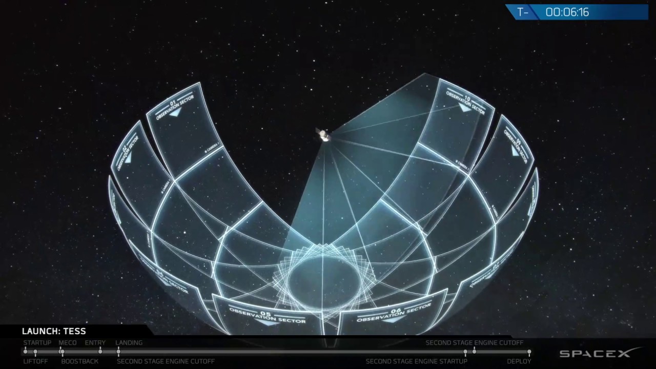
• Why this video: An excellent deep-dive into the launch operations, orbital configuration, and mission design of the Transiting Exoplanet Survey Satellite (TESS). This video shows how TESS's wide-field cameras perform all-sky transit photometry, targeting the nearest and brightest stars.

Could we FINALLY photograph an Earth-like exoplanet?!

@DrBecky16:561200

Could we FINALLY photograph an Earth-like exoplanet?!

A new proposal by Soliman et al. suggests that combining a 99-meter-wide space starshade (a giant umbrella that blocks starlight) with the European Extremely Large Telescope (ELT) could finally enable direct imaging of Earth-like exoplanets, which have been too faint and too close to their stars for current telescopes to detect despite over 6,000 exoplanets having been discovered.

@DrBecky · 16:56

• Why this video: Focuses on the extreme physics of direct imaging. It details the astronomical engineering needed to block out host-star glare, evaluating how space-based "starshades" and ground-based telescopes can combine to resolve faint, rocky planets.

4 Future Space Telescopes NASA wants to build

@LaunchPadAstronomy10:05476699

4 Future Space Telescopes NASA wants to build

Direct imaging of Earth-like exoplanets requires revolutionary technologies to overcome the challenge of planets being 10 billion times fainter than their host stars. HabEx employs two spacecraft: a 4-meter optical telescope with an advanced internal coronagraph and a 52-meter starshade with specially designed petals to eliminate diffraction. The coronagraph blocks most starlight using masks that redirect light to edges, while the starshade provides wide-field mapping capabilities. Precision for

@LaunchPadAstronomy · 10:05

• Why this video: Highlighting NASA's decadal survey pathways, this video covers upcoming flagship optical telescopes designed specifically to find life on exoplanets, focusing on concepts that evolved into the Habitable Worlds Observatory (HWO).

Target Selection and Science Case Simulation for the HWO (Noah Tuchow, UArizona/Steward Observatory)

@originsseminarsandeostalks42643:33471

Target Selection and Science Case Simulation for the HWO (Noah Tuchow, UArizona/Steward Observatory)

The Habitable Worlds Observatory (HWO) represents NASA's next flagship mission following the Roman Space Telescope, serving as a space-based direct imaging observatory designed to detect and characterize Earth-sized planets in the habitable zones of Sun-like stars. The mission aims to characterize atmospheric compositions of approximately 25 exo-Earths by measuring their spectra, functioning essentially as a 'super Hubble' or Hubble 2.0. HWO faces extreme technical challenges requiring planet-st

@originsseminarsandeostalks4264 · 3:33

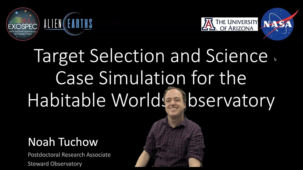
• Why this video: A legitimate scientific research seminar outlining the simulation algorithms and star-selection strategies for the planned $10B+ Habitable Worlds Observatory. It showcases how astronomers model direct imaging targets to maximize biosignature recovery.

Knowledge Checkpoint

• How does TESS's sky coverage and targeted stellar population differ from the original Kepler mission?
• What is a coronagraph, and how does it physically manipulate starlight to reveal companion planets?
• Describe the geometry and alignment of a starshade mission. Why is the starshade deployed tens of thousands of kilometers away from the telescope?
• What is the primary science goal of the Habitable Worlds Observatory (HWO), and what wavelength range will it operate in to detect biosignatures?

Course Map

Key People Index

• Dr. David Kipping (Columbia University / Cool Worlds Lab): Leading exoplanet researcher and educator specializing in the mathematical foundations of radial velocity equations, transit dynamics, and searches for exomoons.
• Prof. Walter Lewin (MIT): Legendary physics educator whose classical mechanics derivations provide the rigorous physical math for waves, binary orbits, and the Doppler effect.
• Dr. Becky Smethurst (Oxford University): Astrophysicist and science communicator who synthesizes complex JWST raw spectra and planetary photochemistry papers into accessible educational material.
• David Charbonneau (Harvard University): Pioneer of transit photometry (mentioned in Module 2/5 references); successfully made the first detection of a transiting exoplanet (HD 209458b) in 1999.
• Dr. Jake Taylor (Oxford/JWST Team): Atmospheric specialist featured in Module 3 who helped lead the analysis of Wasp-39b photochemistry under JWST's Early Release Science Program.
• Prof. Avi Loeb (Harvard University): Astrophysicist known for early orbital and gravitational microlensing research at Princeton, now a leading (and controversial) voice in astrobiology and searches for anomalous cosmic signatures.

Final Self-Assessment

To verify your mastery over modern exoplanet discovery and characterization, you should be able to confidently complete and explain the following physical concepts:

• Draw a complete transit light curve, label the contact points ($t_1, t_2, t_3, t_4$), and explain how to calculate the planet-to-star radius ratio ($\frac{R_p}{R_*}$) using the transit depth.
• Derive a star's radial velocity semi-amplitude using classical Newtonian gravity, and explain why it is harder to detect a lightweight Earth-mass planet at $1 \text{ AU}$ than a massive Jupiter-mass planet at $0.1 \text{ AU}$ (Hot Jupiter).
• Distinguish between an absorption line and an emission line on an exoplanet spectrum plot, and explain what physical parameters determine the baseline continuum.
• State the primary photolysis pathway by which water or hydrogen sulfide is broken down by stellar UV light, and explain how this leads to the formation of sulfur dioxide ($SO_2$) in hot gas giants.
• Mathematically calculate the "habitable zone" boundaries of an active M-dwarf star compared to a G-type star (like our Sun), factoring in the change in stellar luminosity.
• Detail the physical and chemical reason why a co-detection of oxygen ($O_2$) and methane ($CH_4$) in a planet's atmosphere indicates life, explaining why abiotic geology cannot sustain this state.
• Explain the technological limitations of radial velocity instruments (e.g., stellar activity/jitter) and how next-generation spectrographs aim to overcome them to achieve $10 \text{ cm/s}$ precision.
• Contrast the physical light-blocking mechanism of an internal coronagraph with an external starshade, listing the major structural pros and cons of both.