Computational Chemistry: DFT, MM & QM

Learning Goal:
Students will master the fundamentals of Computational Chemistry, moving from classical molecular mechanics and force field formulations to advanced quantum chemical calculations and Density Functional Theory (DFT). By the end of this curriculum, students will possess both the mathematical intuition behind molecular simulations and the practical skills required to run geometry optimizations, perform transition state searches, and interpret thermodynamic output files using state-of-the-art software.

---

Prerequisites

• General Chemistry: Standard chemical bonding, Lewis structures, molecular geometry (VSEPR theory), and thermodynamics.
• Basic Mathematics: Introductory calculus (derivatives, integration) and linear algebra (vectors, matrix transformations).

Estimated Study Time

• Total Estimated Hours: 18 hours (includes video lectures, hands-on tutorials, software practice, and self-assessment).

---

Module 1: Foundations of Molecular Structure & Math

Module Overview

To model a molecule computationally, we must first learn how to mathematically represent its three-dimensional structure and master the physical chemistry math used to solve these systems. This module introduces molecular coordinate systems—contrasting Cartesian space with internal coordinates (Z-matrix format)—and reviews the fundamental physical chemistry math required for computational modeling.

---

Recommended Videos

Video 1: Physical Chemistry Math Fundamentals

Why this video

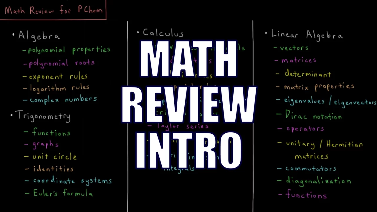
Computational chemistry is highly math-intensive. This video acts as a critical primer, isolating the exact algebraic, trigonometric, and calculus tools needed for physical chemistry calculations. It saves you time by focusing only on the mathematical structures relevant to coordinate transforms and quantum operations.

Knowledge Checkpoint

• Understand the algebraic prerequisites of physical chemistry (quadratics, exponents, logarithms).
• Recall how trigonometric functions (sine, cosine, tangent) map onto molecular coordinate rotations.
• Identify how operators are used as mathematical functions that act upon structures.

---

Video 2: Coordinate Systems & The Z-Matrix

Why this video

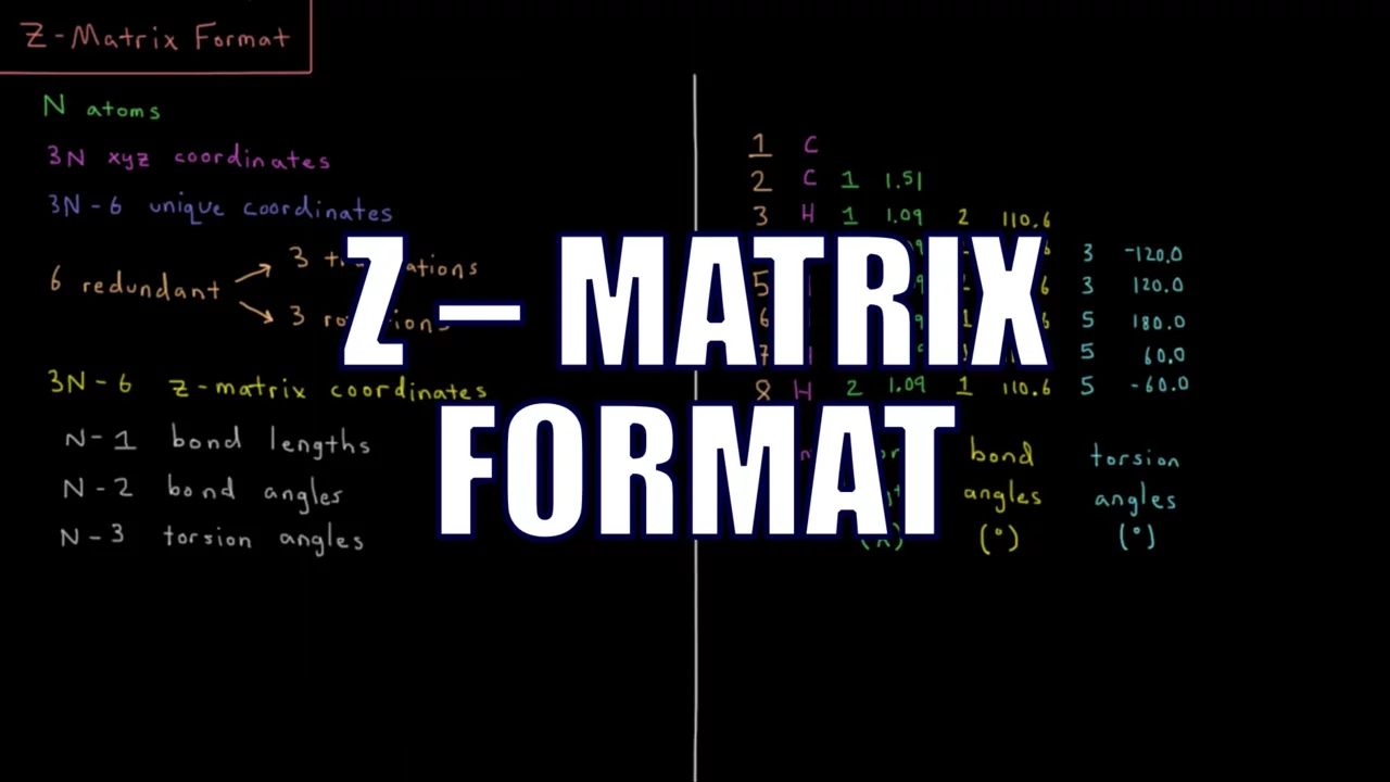
Computers require highly structured coordinate files to calculate atomic forces. While Cartesian ($x, y, z$) coordinates are simple, they contain redundant translational and rotational degrees of freedom (the 6 coordinates describing overall movement). This video details the Z-matrix format, which uses internal degrees of freedom (bond lengths, bond angles, and torsion/dihedral angles) to uniquely define a molecular geometry.

Knowledge Checkpoint

• Differentiate between Cartesian coordinates and internal coordinates.
• Explain how a Z-matrix uses bond lengths ($r$), bond angles ($\theta$), and dihedral angles ($\phi$) to define a molecular structure.
• Write out a basic Z-matrix structure for a simple triatomic molecule like water ($H_2O$).

---

Video 3: Introduction to Molecular Geometry

Why this video

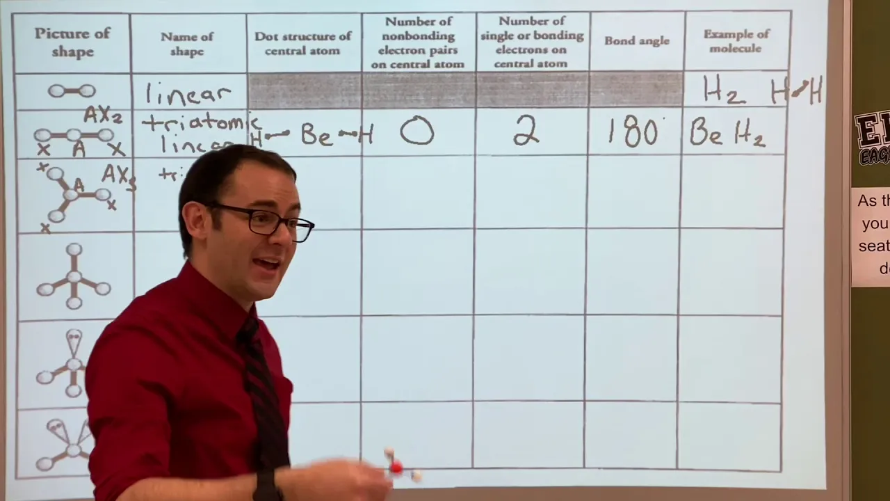
Before optimization algorithms can solve for the lowest-energy molecular state, a physical chemist must have an intuitive starting point. This video reviews fundamental VSEPR theory and the AXE notation system, ensuring you understand the spatial constraints and bond angles that software will refine.

Knowledge Checkpoint

• Use AXE notation to determine the basic geometry (linear, bent, trigonal planar, tetrahedral) of a target molecule.
• Explain how lone electron pairs compress adjacent bonding angles away from idealized values.
• Visualize three-dimensional molecular configurations from structural formulas.

---

Module 2: Molecular Mechanics and Force Fields

Module Overview

Quantum calculations are highly accurate but computationally expensive, scaling poorly with large systems. Molecular Mechanics (MM) circumvents this limit by treating molecules classically—approximating atoms as spheres (masses) and bonds as springs.

This module covers the core mathematical components of classical force fields (bond stretching, angle bending, torsion, and non-bonded interactions) and explores how molecules navigate Potential Energy Surfaces (PES).

Mathematical Formulation of Classical Force Fields

To fully grasp Molecular Mechanics, you must master the fundamental classical force field equation representing total potential energy ($E_{\text{total}}$):

$E_{\text{total}} = E_{\text{stretch}} + E_{\text{bend}} + E_{\text{torsion}} + E_{\text{non-bonded}}$

1. Bond Stretching ($E_{\text{stretch}}$): Modeled using Hooke's Law as a harmonic oscillator: $E_{\text{stretch}} = \sum_{\text{bonds}} \frac{1}{2} k_r (r - r_0)^2$ where $k_r$ is the bond force constant, $r$ is the actual bond length, and $r_0$ is the equilibrium bond length.
2. Angle Bending ($E_{\text{bend}}$): Also modeled harmonically: $E_{\text{bend}} = \sum_{\text{angles}} \frac{1}{2} k_\theta (\theta - \theta_0)^2$ where $k_\theta$ is the bending force constant, $\theta$ is the bond angle, and $\theta_0$ is the equilibrium bond angle.
3. Torsional Rotations ($E_{\text{torsion}}$): Modeled using periodic cosine functions to account for steric barriers: $E_{\text{torsion}} = \sum_{\text{dihedrals}} \frac{V_n}{2} [1 + \cos(n\phi - \gamma)]$ where $V_n$ is the barrier height, $n$ is the multiplicity (periodicity), $\phi$ is the dihedral angle, and $\gamma$ is the phase angle.
4. Non-bonded Interactions ($E_{\text{non-bonded}}$): Typically modeled via the Lennard-Jones 12-6 potential (for van der Waals dispersion and repulsion) and Coulomb's law (for electrostatic charges): $E_{\text{non-bonded}} = \sum_{i < j} \left( 4\epsilon_{ij} \left[ \left(\frac{\sigma_{ij}}{r_{ij}}\right)^{12} - \left(\frac{\sigma_{ij}}{r_{ij}}\right)^6 \right] + \frac{q_i q_j}{4\pi\varepsilon_0 r_{ij}} \right)$

---

Recommended Videos

Video 1: Foundations of the Potential Energy Surface (PES)

Why this video

This lecture by Prof. Christopher Cramer provides an in-depth conceptual breakdown of the Potential Energy Surface (PES). Understanding how molecular coordinates map mathematically to energy is crucial for locating stable configurations (local minima) and chemical transition states (saddle points).

Knowledge Checkpoint

• Define a Potential Energy Surface (PES) and explain how its dimensionality scales with the number of atoms ($3N-6$ or $3N-5$).
• Distinguish between local minima, global minima, and saddle points on a PES.
• Explain how geometry optimization algorithms walk across a PES to find stable structures.

---

Video 2: Force Field Equations (Stretch, Bend, and Torsion)

Why this video

This video explains the classical equations that govern Molecular Mechanics. It introduces Hooke's Law approximations for stretching and bending, and trigonometric expansions for torsional rotations. It provides the direct mathematical framework for the classical potential energy terms detailed in our module overview.

Knowledge Checkpoint

• Explain why a harmonic potential (Hooke's Law) is a good approximation for bond stretching near the equilibrium geometry, and where its physical accuracy fails (e.g., at bond dissociation).
• Describe the physical meaning of the parameters $k_r$, $r_0$, $k_\theta$, and $\theta_0$ in classical mechanics.
• Explain how periodic cosine potentials prevent atom-on-atom overlap during a $360^\circ$ dihedral rotation.

---

Video 3: Force Field Parameters & Scaling

Why this video

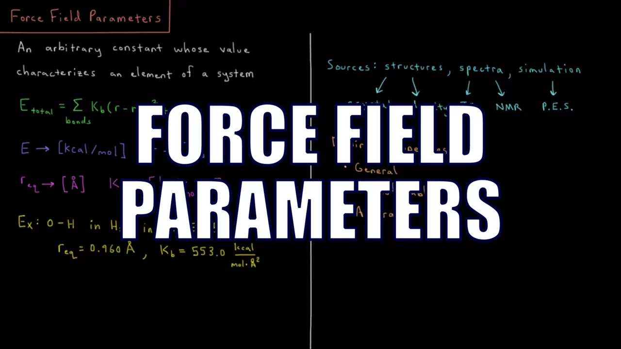
A classical force field equation is useless without parameter values (equilibrium values and force constants) derived from experimental data or high-level quantum calculations. This video explores where these parameters come from and how they define "atom types."

Knowledge Checkpoint

• Define "atom typing" and explain why an $sp^3$ carbon has different parameters than an $sp^2$ carbonyl carbon.
• Discuss the trade-offs of using highly specialized parameter sets versus generic, transferrable force fields (like AMBER, CHARMM, or MM3).
• Explain how non-bonded Lennard-Jones parameters prevent atoms from collapsing into one another.

---

Video 4: Molecular Dynamics Simulations

Why this video

Once we have a classical potential energy function, we can apply Newton's second law of motion ($F=ma$) to calculate atomic trajectories over time. This video provides a high-level overview of Molecular Dynamics (MD) simulations, explaining how statistical mechanics links molecular motion to macroscopic thermodynamic properties.

Knowledge Checkpoint

• Explain how force field derivatives ($F_i = -\nabla_i E$) are used to compute atomic accelerations.
• Describe how Newton's equations of motion are integrated numerically (e.g., using Verlet or Leap-frog algorithms).
• Differentiate between a static geometry optimization and a dynamic MD trajectory.

---

Module 3: Quantum Chemistry & Wave Function Theory

Module Overview

When classical physics fails—such as when bonds form, break, or electrons transition energy levels—we must use quantum mechanics. This module transitions to the quantum realm.

We will unpack the Schrödinger equation, understand how basis sets are used as mathematical toolkits to build electronic configurations, and examine the Hartree-Fock Self-Consistent Field (SCF) method.

---

Recommended Videos

Video 1: Unpacking the Schrödinger Equation

Why this video

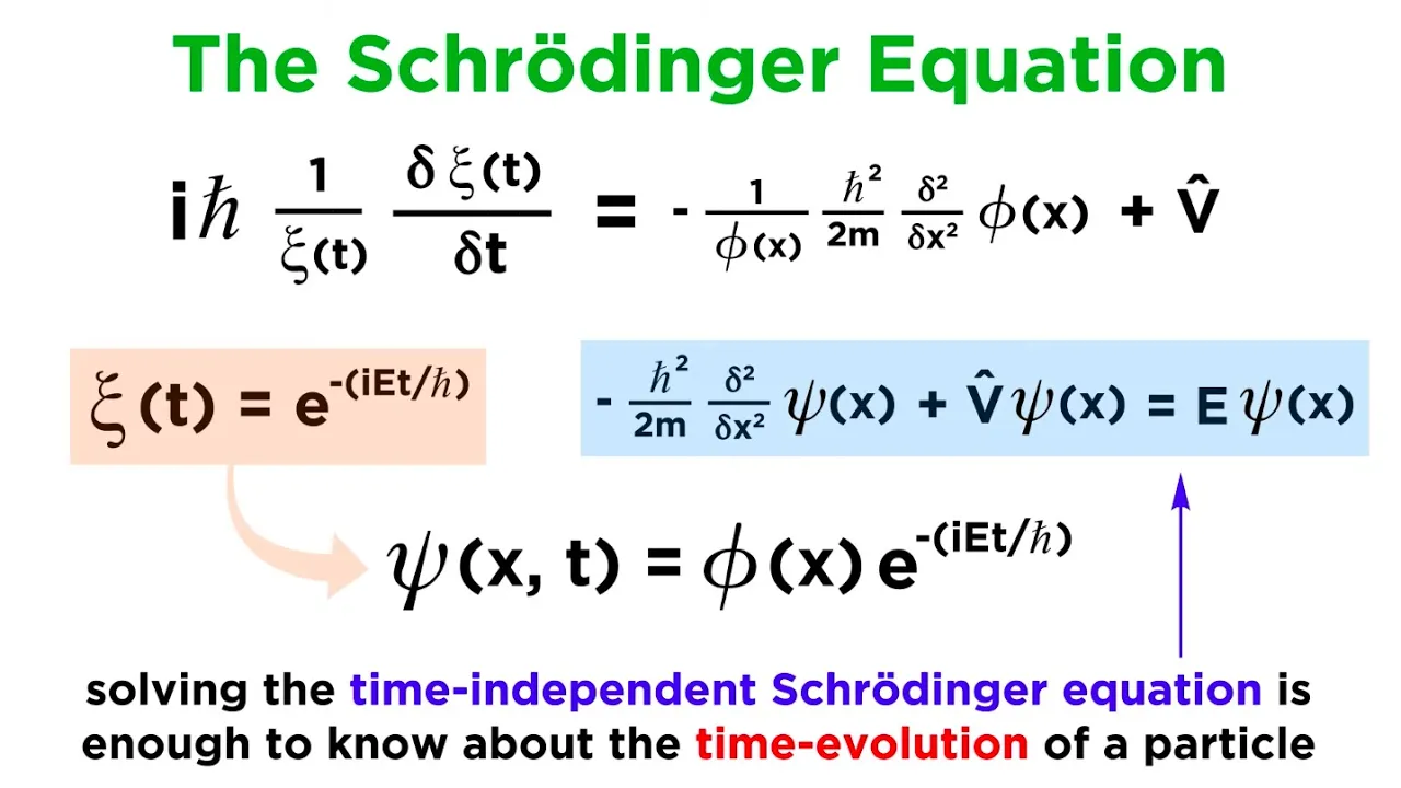
This video breaks down the Time-Independent Schrödinger Equation ($H\Psi = E\Psi$), which is the foundation of quantum chemistry. It explains the physical meaning of the Hamiltonian operator ($H$), the wavefunction ($\Psi$), and eigenvalues ($E$) in an accessible, step-by-step manner.

Knowledge Checkpoint

• State the time-independent Schrödinger equation and label all its mathematical elements.
• Explain the physical meaning of the wavefunction ($\Psi$) and its square amplitude ($|\Psi|^2$, the probability density).
• Define the Hamiltonian operator ($H$) and describe its kinetic and potential energy components.

---

Video 2: Introduction to Basis Sets

Why this video

In computational chemistry, we cannot solve the Schrödinger equation exactly for multi-electron systems. Instead, we approximate wavefunctions using linear combinations of pre-defined mathematical functions called basis sets. This MIT OCW lecture explains basis sets and how choosing different levels of mathematical refinement affects computational cost and accuracy.

Knowledge Checkpoint

• Define a basis set and explain why it is essential for solving the electronic Schrödinger equation.
• Differentiate between Slater-Type Orbitals (STOs) and Gaussian-Type Orbitals (GTOs).
• Understand split-valence notation (e.g., how Pople's 6-31G* basis set uses different numbers of Gaussian functions for core and valence shells).

---

Video 3: Molecular Orbital (MO) Theory

Why this video

This MIT lecture details how atomic orbital wavefunctions are combined (Linear Combination of Atomic Orbitals, or LCAO) to build delocalized molecular orbitals. This provides the chemical framework needed to understand bonding, anti-bonding, and electronic configurations.

Knowledge Checkpoint

• Describe the LCAO approximation and how constructive vs. destructive interference creates bonding and anti-bonding orbitals.
• Sketch simple molecular orbital diagrams for homonuclear diatomic molecules ($H_2$, $N_2$).
• Explain how MO theory accounts for orbital delocalization across a molecule, unlike traditional localized Lewis structures.

---

Video 4: The Hartree-Fock Self-Consistent Field (SCF) Method

Why this video

The multi-electron Schrödinger equation cannot be solved exactly because electrons interact with and repel each other. Hartree-Fock theory handles this by assuming each electron moves within an average electrostatic field created by all other electrons. This lecture shows how this "circular" problem is solved iteratively using the Self-Consistent Field (SCF) approach.

Knowledge Checkpoint

• Explain the "many-body problem" and why electron-electron repulsion terms complicate quantum calculations.
• Detail the iterative steps of the Self-Consistent Field (SCF) method (guess orbital coefficients, build Hamiltonian, solve, repeat until energy converges).
• Define a Slater determinant and explain how it satisfies the Pauli exclusion principle (antisymmetry of the wavefunction).

---

Module 4: Density Functional Theory (DFT)

Module Overview

Hartree-Fock is highly structured but omits electron correlation (how electrons dynamically avoid each other). Doing so makes it chemically inaccurate for many systems unless expensive corrections are added.

Density Functional Theory (DFT) offers an alternative approach: instead of solving for a complex $3N$-dimensional wavefunction (for $N$ electrons), DFT proves that the total ground-state energy can be calculated directly from the $3$-dimensional electron probability density $\rho(\mathbf{r})$. This module covers the foundational theorems, equations, and functional approximations that make DFT the most widely used tool in computational chemistry.

---

Recommended Videos

Video 1: The Hohenberg-Kohn Theorems

Why this video

This lecture by Prof. Christopher Cramer addresses a common gap in computational chemistry courses: a clear, conceptual explanation of the physical proofs behind DFT. It covers the first and second Hohenberg-Kohn theorems, establishing the mathematical validity of using electron density to solve molecular systems.

Theoretical Core: The Hohenberg-Kohn Theorems

1. The First Hohenberg-Kohn Theorem: Proves that the ground-state electron density $\rho(\mathbf{r})$ uniquely determines the external potential $V_{\text{ext}}(\mathbf{r})$ (up to an additive constant). Because the external potential uniquely defines the Hamiltonian, the ground-state density uniquely determines all quantum properties of the system.
2. The Second Hohenberg-Kohn Theorem: Establishes a variational principle for density. It proves that for any trial density $\tilde{\rho}(\mathbf{r})$ that is positive and integrates to the correct number of electrons: $E[\tilde{\rho}] \geq E_0[\rho_0]$ where $E_0$ is the true ground-state energy. This guarantees that minimizing the energy functional with respect to density will yield the exact ground-state density and energy.

Knowledge Checkpoint

• State and explain the physical significance of the first Hohenberg-Kohn theorem.
• Explain how the second Hohenberg-Kohn theorem enables computational software to find the ground state using variational optimization.
• Define a "functional" (a mathematical operator that takes a function, like electron density, and maps it to a single scalar value, like energy).

---

Video 2: The Kohn-Sham Equations

Why this video

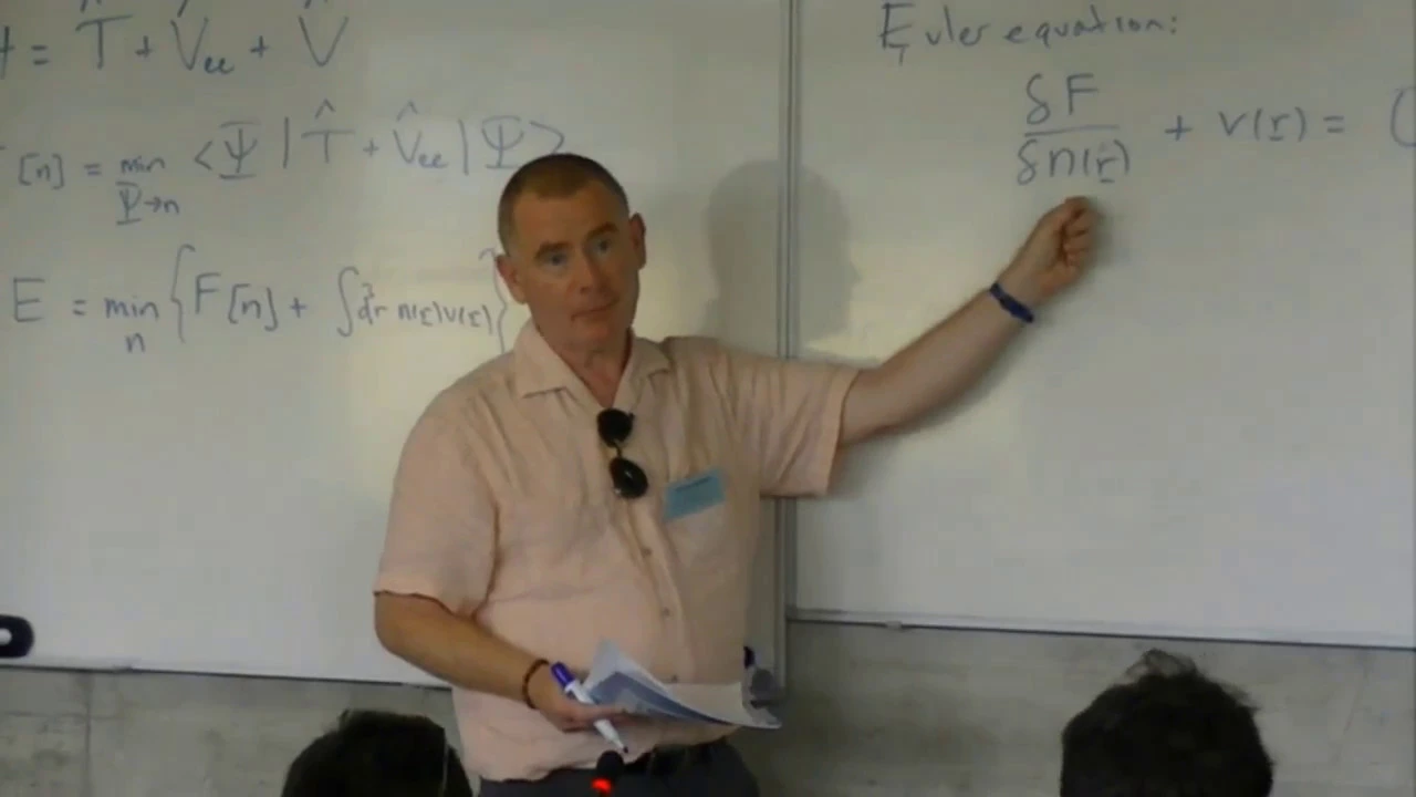
While the Hohenberg-Kohn theorems prove a direct relationship between density and energy exists, they do not provide a practical way to calculate the kinetic energy of interacting electrons. Kohn and Sham solved this by introducing a fictitious reference system of non-interacting electrons that yields the exact same spatial density. This extensive lecture details how these equations form the practical engine of modern DFT.

Knowledge Checkpoint

• Explain how the Kohn-Sham approach simplifies the calculations by splitting the kinetic energy functional into a major non-interacting term and a minor correction term.
• Write out the Kohn-Sham equation, detailing the effective potential $V_{\text{eff}}(\mathbf{r})$ which includes Hartree and exchange-correlation potentials.
• Discuss how the Kohn-Sham self-consistent loop mirrors the Hartree-Fock SCF method.

---

Video 3: Exchange-Correlation Functionals

Why this video

In Kohn-Sham DFT, all complex quantum interactions—including exchange, correlation, and kinetic energy corrections—are grouped into a single, unknown term: the Exchange-Correlation functional ($E_{\text{xc}}[\rho]$). This video reviews the "Jacob's Ladder" of density functional approximations, helping you select the appropriate functional (e.g., LDA, GGA, or Hybrid functionals like B3LYP) for your calculations.

Knowledge Checkpoint

• Describe the Local Density Approximation (LDA) and identify the systems where it is most accurate (e.g., uniform electron gases).
• Explain how Generalized Gradient Approximations (GGAs) improve upon LDA by incorporating the local gradient of the density ($\nabla\rho$).
• Define "hybrid functionals" (such as B3LYP) and explain why mixing in a fraction of exact Hartree-Fock exchange energy improves chemical accuracy.

---

Module 5: Practical Quantum Chemical Calculations

Module Overview

This module connects theory to practice. Here, you will learn to build molecules in a graphical user interface (Avogadro), generate calculation inputs for modern electronic structure packages (such as ORCA or Gaussian), run geometry optimizations, and analyze output files.

We will pay close attention to evaluating vibrational frequencies (to confirm stable states vs. transition states) and calculating thermodynamic values (such as Enthalpy and Gibbs free energy).

Practical Guide: Interpreting Calculation Output Files

When your calculation finishes, it yields a massive text file (typically a .out or .log file). To extract meaningful chemistry from it, you must locate several key sections:

1. Geometry Optimization Convergence

Verify that the geometry search converged successfully. In the output, look for a criteria block that should display all converged values:

*** GEOMETRY OPTIMIZATION CYCLE CONVERGED ***

If the calculation terminated because it ran out of steps rather than converging, your structure is invalid, and you should check your starting coordinates.

2. Vibrational Frequency Analysis & Transition States

Running a frequency calculation allows you to characterize the nature of your stationary point on the PES:

• Stable Intermediate (Local Minimum): All calculated vibrational frequencies must be real numbers (reported as positive values). This indicates that moving any atom in any direction increases the potential energy.
• Transition State (TS): Your frequency analysis must yield exactly one imaginary frequency (often printed as a negative number, e.g., -342 cm⁻¹ or labeled with i). This imaginary frequency corresponds to the transition vector along the reaction coordinate. If you have two or more imaginary frequencies, your structure is a high-order saddle point rather than a valid physical transition state.

3. Thermodynamic Enthalpy and Gibbs Free Energy Corrections

A standard DFT geometry optimization calculates the electronic energy at $0\text{ K}$ without molecular motion. To compare your results with experimental laboratory conditions ($298.15\text{ K}$, $1\text{ atm}$), you must calculate thermodynamic corrections derived from vibrational partition functions. Search your output file for these thermodynamic values:

• Zero-Point Energy (ZPE): The fundamental vibrational energy remaining at absolute zero.
• Enthalpy (H): Usually printed as Total Enthalpy or Sum of electronic and thermal Enthalpies ($H(T) = E_{\text{electronic}} + \text{ZPE} + E_{\text{thermal\_corrections}} + k_B T$).
• Gibbs Free Energy (G): Usually listed as Final Gibbs Free Energy or Sum of electronic and thermal Free Energies ($G(T) = H(T) - TS(T)$). Use this value to compute thermodynamic reaction energies ($\Delta G_{\text{rxn}}$) and activation barriers ($\Delta G^{\ddagger}$).

---

Recommended Videos

Video 1: Building Molecules in Avogadro

Why this video

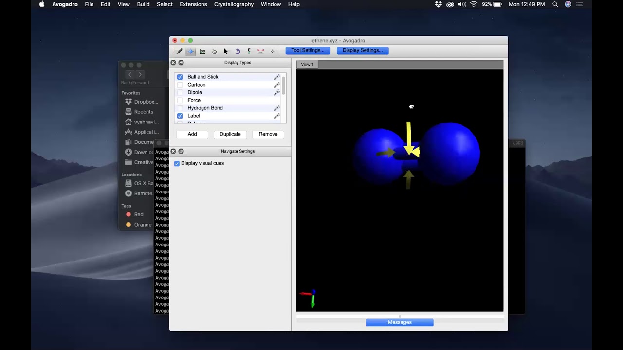
This practical guide walks you through building three-dimensional chemical structures in Avogadro. It covers drawing bonds, adjusting elements, applying force-field pre-optimizations to relax starting geometries, and formatting coordinates for quantum calculation inputs.

Knowledge Checkpoint

• Use the draw tool to construct organic and inorganic structures with proper valence bonds.
• Apply the built-in force-field geometry tool (such as UFF or MM94) to pre-optimize coordinates before submitting them to quantum engines.
• Export coordinates from Avogadro as an input structure (.xyz or .pdb format).

---

Video 2: Running Geometry Optimizations in ORCA

Why this video

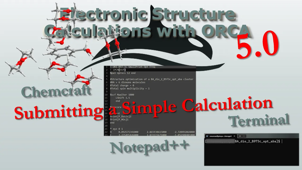
This video details the process of taking your built coordinates and setting up an ORCA input file. It explains key commands like charge and multiplicity, functional selection, basis set choice, and running the calculation.

Knowledge Checkpoint

• Construct a basic ORCA input file (.inp) with the correct block formatting.
• Determine the correct total charge and spin multiplicity ($2S+1$) for your target molecule.
• Differentiate between a single point energy calculation (SP) and a geometry optimization calculation (Opt).

---

Video 3: Vibrational Frequency Calculations

Why this video

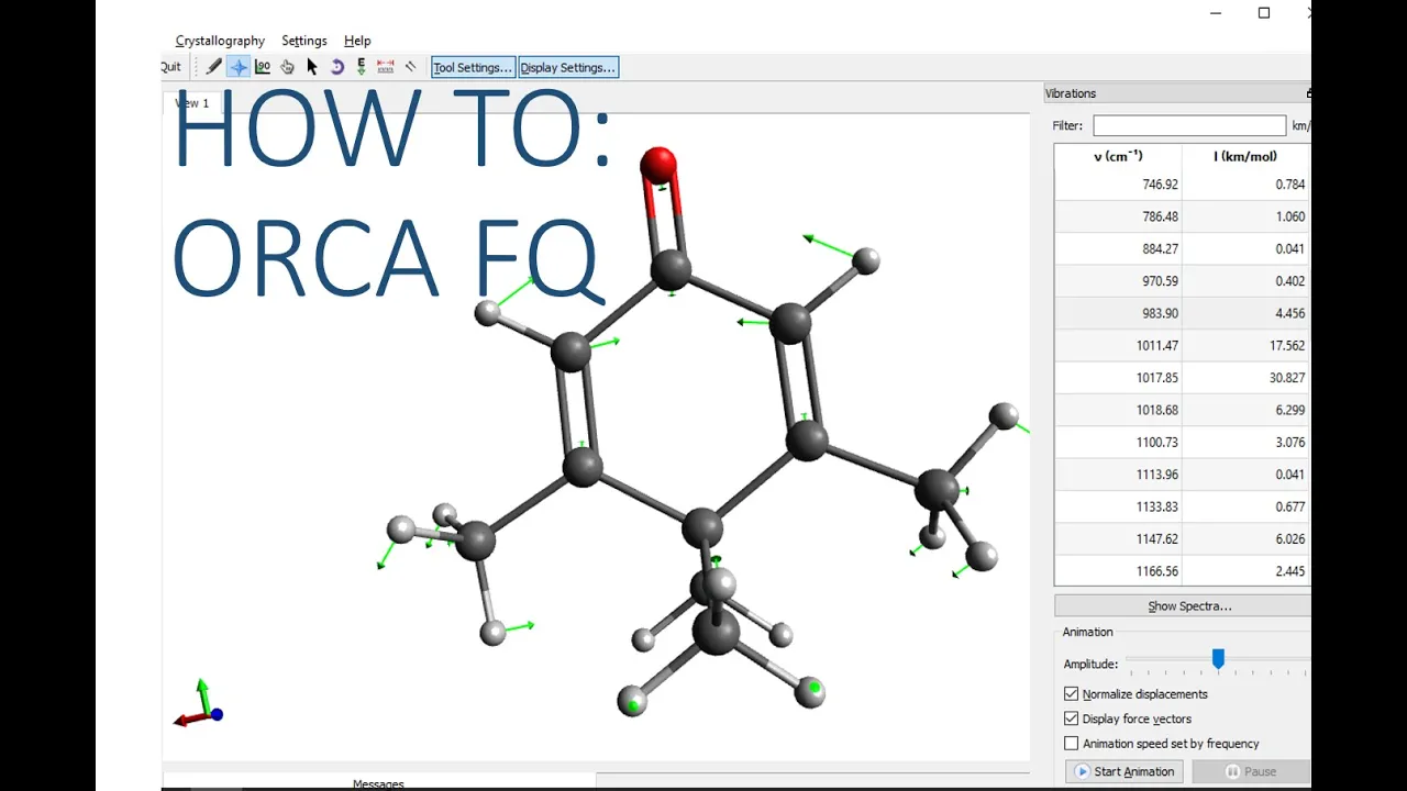
To calculate vibrational frequencies, software must compute the Hessian matrix (second derivatives of energy with respect to nuclear displacement). This video shows how to run frequency calculations in ORCA, visualize vibrational modes, and extract thermodynamic values.

Knowledge Checkpoint

• Explain why a frequency calculation must always be performed on an already-optimized geometry rather than an unrelaxed starting coordinate.
• Open an ORCA output file in a visualizer and animate vibrational modes (e.g., carbonyl stretches).
• Identify the location of zero-point energies, thermal enthalpy corrections, and Gibbs free energy values in the output text.

---

Video 4: Finding Transition States of Reactions

Why this video

Finding reaction pathways requires locating saddle points on the PES that connect reactants to products. This comprehensive tutorial walks you through setting up transition state calculations, performing optimization searches, and verifying your results using frequency analysis.

Knowledge Checkpoint

• Construct a starting guess for a transition state using intermediate bond-forming/bond-breaking lengths.
• Set up a Transition State optimization (OptTS) calculation in ORCA.
• Confirm a successful TS search by finding exactly one imaginary frequency, and animate that mode to verify it describes the correct reaction pathway.

---

Course Map

Below is the recommended pathway through the curriculum modules. Ensure you complete Module 1 and understand coordinate representations before moving on to either Module 2 (Classical mechanics pathway) or Module 3 (Quantum mechanics pathway).

---

Key People Index

• Erwin Schrödinger (1887–1961): Formulated the fundamental wave equation of quantum mechanics, describing physical systems through wavefunctions.
• Douglas Hartree (1897–1958) & Vladimir Fock (1898–1974): Developed the Hartree-Fock self-consistent field approximation method, which provides a starting point for solving many-body electronic structures.
• Pierre Hohenberg (1934–2017) & Walter Kohn (1923–2016): Proved the Hohenberg-Kohn theorems, establishing that all ground-state electronic properties can be calculated using only the electron density. Kohn was awarded the 1998 Nobel Prize in Chemistry for this work.
• Lu Jeu Sham (1938–present): Developed the Kohn-Sham equations alongside Walter Kohn, transforming density functional theory into a practical computational tool.
• Christopher Cramer (1961–present): Professor and author of Essentials of Computational Chemistry, a major figure in making quantum chemical education accessible.

---

Final Self-Assessment

Test your understanding of the theoretical and practical concepts covered across all modules.

• Coordinate systems: Explain why Cartesian coordinate files are typically used as input structures, but optimization software often converts them to internal coordinates (Z-matrix format) during calculation loops.
• Force Field math: Write down the mathematical term for a Hooke's Law approximation of bond stretching and explain why it fails to model bond cleavage.
• Potential Energy Surfaces: Distinguish between a transition state (saddle point) and a stable intermediate (local minimum) on a multidimensional Potential Energy Surface.
• The Schrödinger equation: Write the time-independent Schrödinger equation and define the role of the Hamiltonian operator.
• Hartree-Fock SCF: Explain the term "Self-Consistent Field" and detail why an iterative computational loop is required to solve the Hartree-Fock equations.
• Basis Sets: Define split-valence basis sets and explain why polarizable functions (like the '' in 6-31G) are necessary when modeling polar molecules or lone pairs.
• The Hohenberg-Kohn Theorems: State the first Hohenberg-Kohn theorem and explain how it shifts the focus from many-body wavefunctions to 3D electron densities.
• The Kohn-Sham approach: Describe how Kohn-Sham equations handle kinetic energy by introducing a reference system of non-interacting electrons.
• Functionals: Identify the differences between LDA, GGA, and Hybrid functionals, and choose which family you would use to calculate a complex reaction barrier.
• Calculations: Explain why you must always run a frequency calculation after completing a geometry optimization.
• Transition States: Detail how to verify whether an optimized structure is a true transition state, a stable intermediate, or an invalid higher-order saddle point.
• Thermodynamics: Describe how to extract the enthalpy and Gibbs free energy at $298.15\text{ K}$ from an ORCA or Gaussian output file.