Bayesian Inference: Priors, Conjugacy & MCMC
Learning Goal: Construct prior-to-posterior transitions, analyze and derive conjugate priors (such as Beta-Binomial and Normal-Normal models), and design and evaluate Markov Chain Monte Carlo (MCMC) samplers to perform exact and approximate probabilistic modeling.
- Prerequisites: Basic multi-variable calculus (integration), linear algebra, and introductory Python programming (knowledge of NumPy is helpful).
- Estimated Study Time: 32 hours
Module 1: Probability Foundations & Bayes' Theorem
This module establishes the foundational probability theory required for Bayesian statistics. You will study conditional probability, visual interpretations of updating beliefs, and the formal mathematical derivation of Bayes' Theorem.
Recommended Videos

Why this video: This video provides a geometric and visual intuition of Bayes' theorem using area models. It helps build a conceptual foundation before you dive into the algebraic representations of updating beliefs under uncertainty.
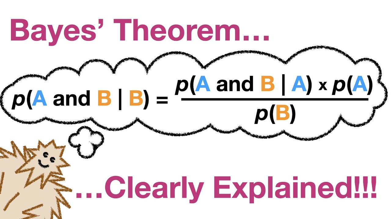
Why this video: StatQuest provides a clear, step-by-step mathematical derivation of Bayes' Theorem. This video bridges the gap between the geometry shown by 3Blue1Brown and the formal notation used in statistical modeling.
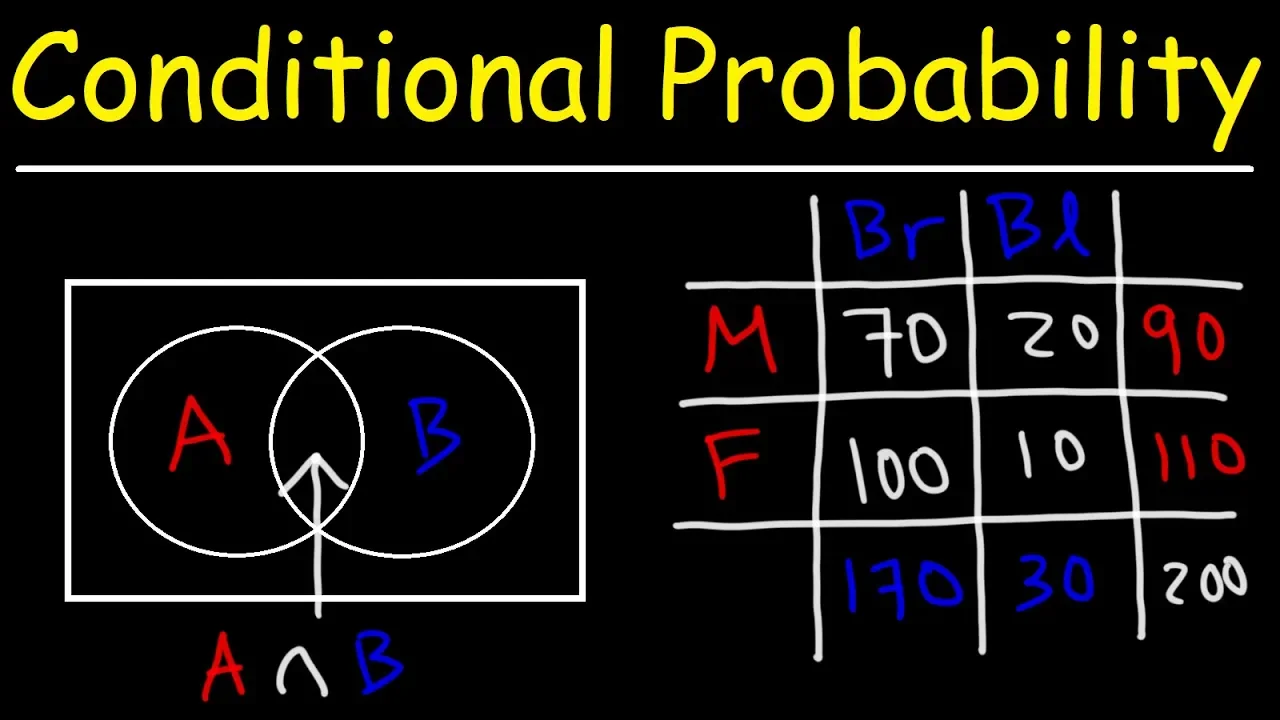
Why this video: This short video offers a rapid, highly intuitive guide to calculating conditional probability using visual tools like Venn Diagrams and joint contingency tables.
Module 1 Knowledge Checkpoint
- Write down the algebraic formula for Bayes' Theorem and label the Prior, Likelihood, Posterior, and Marginal Likelihood (Evidence).
- Explain how a change in the sample space (conditioning on event ) affects the denominator when computing conditional probability .
- Draw a Venn diagram representing two intersecting dependent events and compute given and .
Module 2: Probability Distributions & Likelihood
To work with statistical models, you must understand the distinction between discrete and continuous random variables, probability density functions (PDFs), and the key conceptual differences between probability and likelihood.
Recommended Videos
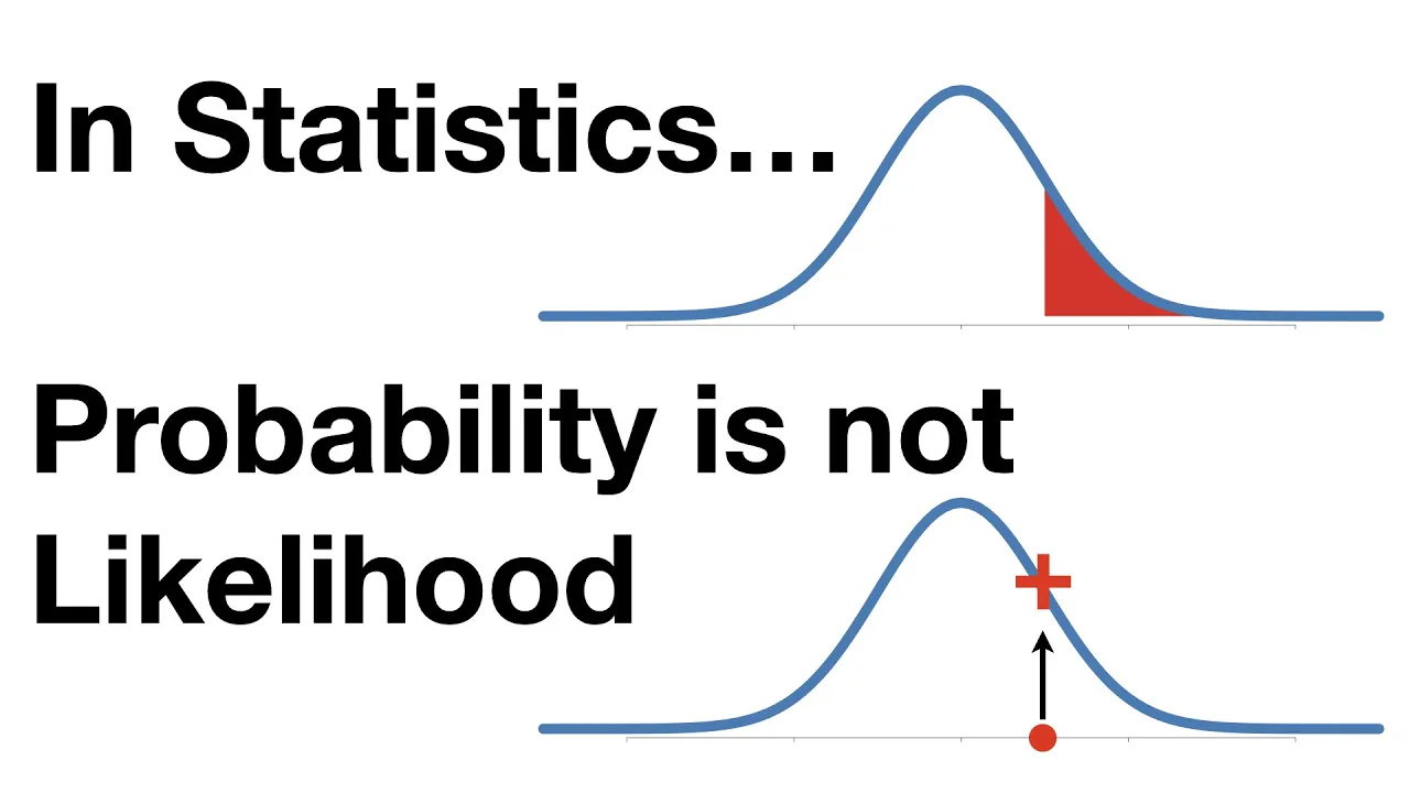
Why this video: One of the most common confusions in statistical inference is mixing up probability and likelihood. StatQuest clarifies this distinction, explaining how probability deals with finding the area under a fixed distribution, while likelihood varies parameters for a fixed dataset.
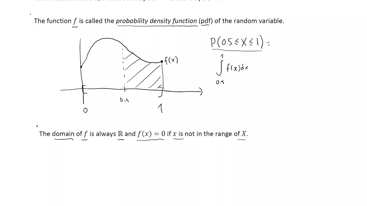
Why this video: This lecture covers continuous random variables and how probability density functions behave. It is essential preparation for handling continuous parameters in Bayesian inference.
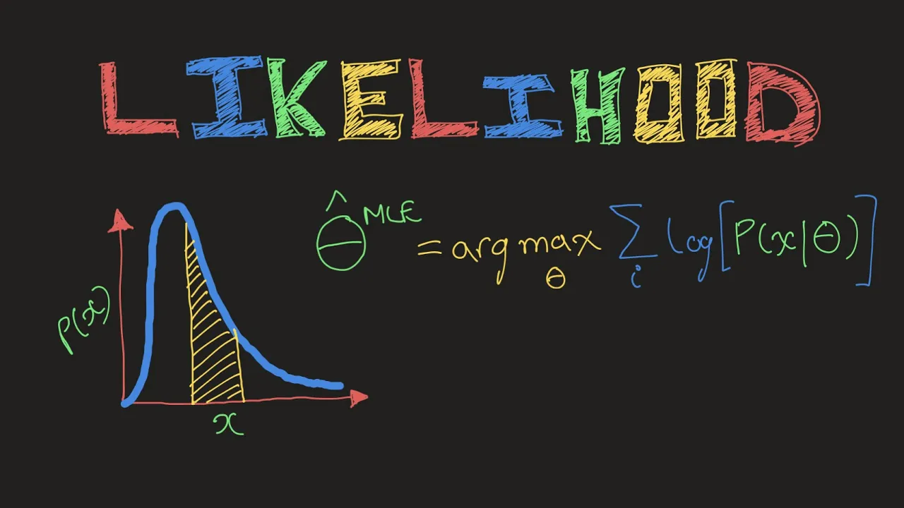
Why this video: This video provides a rigorous breakdown of likelihood functions. It explains how to construct joint likelihood functions mathematically for independent, identically distributed (i.i.d.) observations.
Module 2 Knowledge Checkpoint
- Explain why the probability of a single point in a continuous distribution, , is always zero, and how we use PDFs to calculate interval probabilities.
- Given a probability density function , explain what is held constant and what varies when evaluating it as a probability vs. evaluating it as a likelihood.
- Write the joint likelihood function for independent, identically distributed (i.i.d.) normal observations.
Module 3: The Bayesian Framework: Prior to Posterior
This module introduces the Bayesian paradigm: treating parameters as random variables rather than fixed values. You will explore how prior distributions are systematically updated by the likelihood of observed data to yield a posterior distribution.
Recommended Videos

Why this video: Part of MIT's open curriculum, this rigorous lecture introduces the formal framework of Bayesian inference, laying out the transition from prior to posterior using solid mathematical foundations.
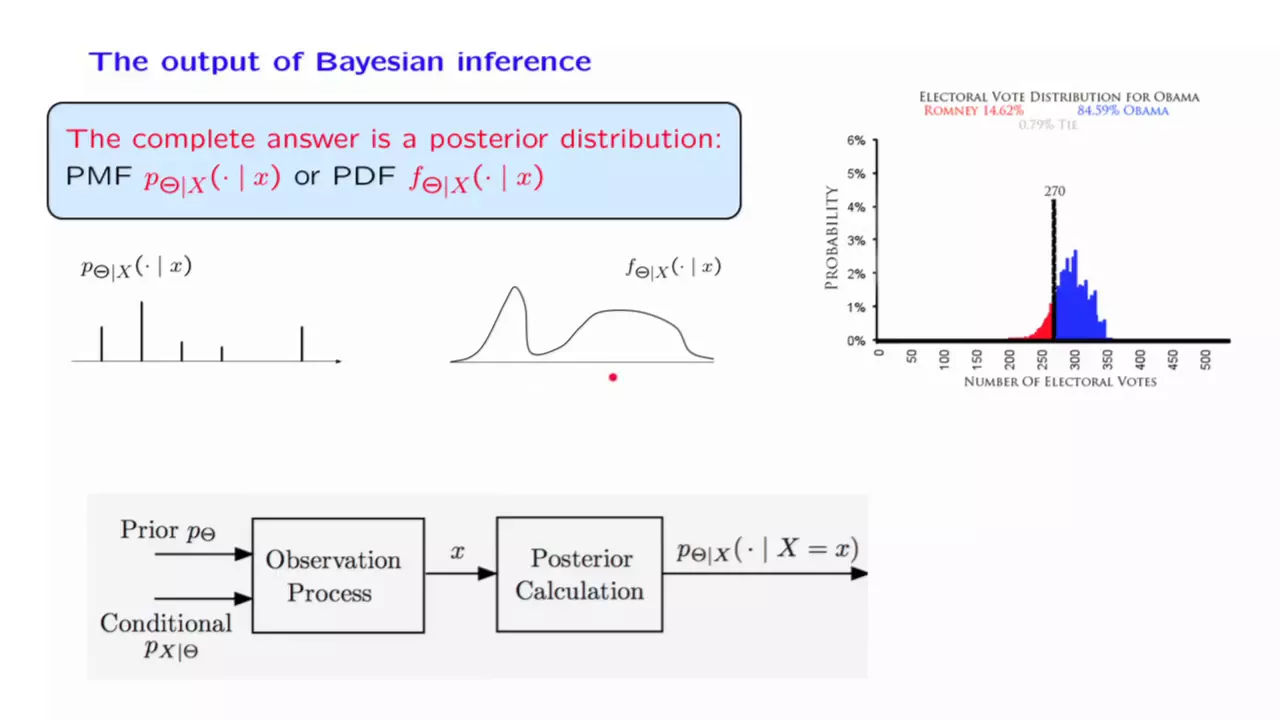
Why this video: A concise distillation from MIT that guides you through the components of Bayesian updating, summarizing how prior beliefs are adjusted as new data points arrive.

Why this video: Mathematical Monk provides a clean, concrete illustration of Bayesian updating, showing how a discrete parameter's distribution shifts after introducing a basic dataset.
Module 3 Knowledge Checkpoint
- Describe the primary philosophical difference between Bayesian inference and Frequentist inference regarding parameters.
- Mathematically state why the posterior distribution is proportional to the product of the prior and the likelihood: .
- Explain the role of the marginal likelihood (the denominator in Bayes' theorem) and explain why it is often referred to as the normalizing constant.
Module 4: Conjugate Priors & Analytical Inference
When the posterior distribution belongs to the same probability family as the prior distribution, the prior is called "conjugate" to the likelihood. This allows you to bypass complex integration and compute posteriors analytically.
Note: The feedback pointed out a lack of step-by-step mathematical derivations in general conjugate overviews. We have solved this below by selecting specialized videos that walk through the detailed math of both Beta-Binomial and Normal-Normal conjugate models.
Recommended Videos

Why this video: An excellent, mathematically sound introduction to the definition and mechanics of conjugate priors, showing why they are useful for analytical Bayesian calculations.

Why this video: Despite its general name, this video directly addresses a key curriculum gap by demonstrating the mathematical derivation of the Beta-Binomial conjugate model. It shows exactly how the prior exponents and likelihood combinatorics combine to form a new Beta distribution.

Why this video: This video provides a step-by-step mathematical walkthrough of updating a Beta prior with Binomial and Bernoulli likelihoods, reinforcing the algebraic steps needed to find posterior hyper-parameters.
![[Bayesian inference for a mean] Unknown mean posterior derivation](https://i.ytimg.com/vi_webp/Qv4oNR3KJN0/maxresdefault.webp)
Why this video: This video addresses our second curriculum gap by providing a step-by-step mathematical derivation of a Normal posterior from a Normal prior and a Normal likelihood. It carefully shows how to complete the square in the exponent.

Why this video: This video reinforces Normal-Normal conjugacy, focusing on how the precision (inverse variance) of the posterior is simply the sum of the prior precision and the data likelihood precision.
Module 4 Knowledge Checkpoint
- Derive the posterior distribution for a prior and a likelihood. Show that the posterior is .
- Define what a "conjugate prior" is and explain the mathematical advantages of using one.
- For a Normal-Normal conjugate model, if your prior variance decreases (representing stronger prior beliefs), how does this affect the posterior mean relative to the sample mean?
Module 5: Markov Chain Monte Carlo (MCMC) & Metropolis-Hastings
In complex probabilistic models, calculating the marginal likelihood analytically is often impossible. This module covers Markov Chain Monte Carlo (MCMC) methods, focusing on how the Metropolis-Hastings algorithm allows us to sample from intractable posterior distributions.
Recommended Videos
Why this video: Dr. Ben Lambert provides a brilliant, clear explanation of why multidimensional integration fails in complex Bayesian models and why we need simulation techniques like MCMC.

Why this video: This video breaks down the Metropolis-Hastings algorithm step-by-step. It explains proposal distributions, acceptance ratios, and how the algorithm explores a parameter space without needing to compute the denominator of Bayes' Theorem.

Why this video: This video provides a clear mathematical explanation of the Metropolis-Hastings algorithm, making it easy to understand the core formulas behind proposal distributions and acceptance probabilities.
Module 5 Knowledge Checkpoint
- Explain why computing the marginal likelihood becomes mathematically intractable when has many dimensions.
- Write the mathematical expression for the Metropolis-Hastings acceptance probability .
- Describe the difference between a symmetric proposal distribution (Metropolis algorithm) and an asymmetric proposal distribution (Metropolis-Hastings algorithm).
Module 6: Gibbs Sampling & Probabilistic Programming
This module explores Gibbs Sampling, a special case of the Metropolis-Hastings algorithm where parameters are updated one by one using their full conditional distributions. You will also learn how to build Bayesian models using Python and R libraries like PyMC and Stan.
Recommended MCMC Diagnostics Guide (Addressing the Video Gap)
The video pool lacks coverage of MCMC convergence diagnostics. To bridge this gap, study the following key diagnostic metrics, which are essential for verifying your samplers before drawing conclusions:
- Traceplots: Time-series plots of your parameter values across sampling steps. A healthy, converged chain looks like a stationary "fuzzy caterpillar." Flat lines or drifting trends suggest poor mixing.
- Gelman-Rubin Diagnostic ( / R-hat): Compares the variance between multiple independent chains to the variance within the chains. A converged model should have (ideally ). If , your chains have not converged to the same distribution.
- Autocorrelation: Measures how correlated successive samples are. High autocorrelation means your sampler is exploring slowly and needs more steps to yield independent samples.
- Effective Sample Size (ESS): Estimates the number of independent samples your highly correlated chain is actually equivalent to.
Recommended Videos

Why this video: This video introduces Gibbs sampling, explaining how to sample from joint multivariate distributions by iteratively drawing from conditional univariate distributions.
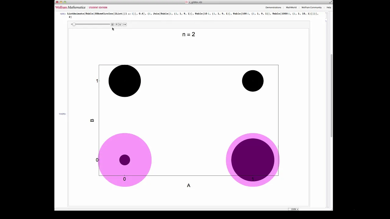
Why this video: A comprehensive and mathematically detailed tutorial on the mechanics of Gibbs sampling. It walks you through a complete bivariate discrete example, showing how the math works step-by-step.
![[41] Intro to Probabilistic Programming with PyMC (Austin Rochford)](https://i.ytimg.com/vi/Qu6-_AnRCs8/maxresdefault.jpg)
Why this video: This video introduces probabilistic programming in Python using PyMC. It shows how to translate theoretical math into computer code that automates Bayesian updating.
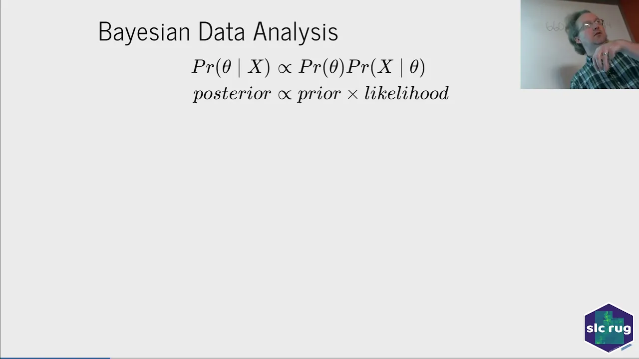
Why this video: A deeper look at Bayesian programming using Stan. This presentation explains how to define priors, likelihoods, and parameter constraints within a production-grade probabilistic programming library.
Module 6 Knowledge Checkpoint
- Explain how Gibbs sampling can be considered a special case of the Metropolis-Hastings algorithm where the acceptance probability is always 1.
- Given a bivariate distribution , outline the exact pseudocode steps for running a Gibbs sampler.
- Identify a "fuzzy caterpillar" traceplot vs. a poorly mixing traceplot, and state what an value of indicates about your model's convergence.
- Write a simple script using a probabilistic programming library (like PyMC or Stan) to estimate the mean and standard deviation of a normal distribution.
Course Map
This flowchart maps the structure of the course, showing module dependencies and the recommended learning path.
Key People Index
- Thomas Bayes (1701–1761): An English statistician and Presbyterian minister who formulated the foundational theorem of conditional probability that bears his name.
- Michael Betancourt: A leading applied statistician and core developer of Stan, known for his work on the geometry and mathematical foundations of Hamiltonian Monte Carlo (HMC).
- Osvaldo Martin: A prominent Bayesian researcher and core developer of PyMC and ArviZ, widely known for his books and educational efforts in probabilistic programming.
- Austin Rochford: An applied mathematician and PyMC contributor who writes extensively on leveraging probabilistic programming for real-world data science.
Final Self-Assessment
Test your understanding of the concepts covered in this curriculum:
- I can derive Bayes' Theorem from the definition of conditional probability: .
- I can explain the mathematical and conceptual differences between probability (area under a curve) and likelihood (height of a curve).
- I can write out the prior, likelihood, and posterior setup for a coin-flipping experiment (Beta-Binomial) and solve for the posterior analytically.
- I can state the conjugate prior families for Poisson, Binomial, and Normal likelihoods.
- I can explain why the marginal likelihood (the denominator of Bayes' Theorem) is computationally intractable in high dimensions, creating the need for simulation.
- I can write the pseudocode for the Metropolis-Hastings algorithm, including the candidate generation and acceptance/rejection steps.
- I can describe how a Gibbs sampler works by iteratively sampling from full conditional distributions.
- I can list and explain the four main MCMC convergence diagnostics: Traceplots, Gelman-Rubin (), Autocorrelation, and Effective Sample Size (ESS).
- I can write a working model in PyMC or Stan to estimate the posterior of parameters from a real dataset and run MCMC sampling on it.