Visualizing Chaos: Dynamics & Fractals
Learning Goal: Visualizing Chaos: Understanding dynamical systems, bifurcation theory, and fractal geometry through differential equations.
This curriculum takes you on a visual journey from the basic calculus of change to the stunning, infinite complexity of chaotic systems. You will learn to see equations not as dry strings of algebra, but as living, geometric structures that bend, warp, split, and fracture.
- Prerequisites: High school algebra and an intuitive understanding of coordinates. No advanced calculus background is required; all geometric concepts are introduced visually.
- Estimated Total Study Time: 16 hours
Module 1: Foundations of Differential Equations & State Space
This module provides a visual entry point into the mathematics of change. Instead of focusing on symbolic integration techniques, you will learn to interpret differential equations geometrically. We will conceptualize state space (or phase space)—a coordinate system where every point represents a complete snapshot of a system's state—and see how system rules generate vector fields and trajectories.
Recommended Videos

Why this video
This video demystifies what a differential equation actually is. By using clear, real-world dynamics like velocity (the first derivative of position) and acceleration (the second derivative), it builds an intuitive bridge between physical change and mathematical equations without drowning you in abstract proofs.

Why this video
Presented by world-renowned mathematician Steven Strogatz, this brief introduction defines the core philosophy of our study: phase space. Strogatz explains how states map to geometric points and how solutions correspond to moving trajectories, setting up a spatial framework for analyzing complex behavior.

Why this video
This video offers a clean, zero-calculus visualization of how different initial conditions yield distinct trajectories in a phase plane. It demonstrates how a collective family of these trajectories forms a complete phase portrait, allowing you to read a system's global behavior at a glance.
Gap Recommendation: If you struggle to visualize how vector fields translate directly to trajectories, try searching YouTube for "Vector fields and phase portraits visual introduction" or explore the interactive "Desmos phase portrait simulator" to plot your own custom coordinate curves in real time.
Knowledge Checkpoint
- Can you define "state space" and explain how a single point represents a physical system?
- What is the difference between an individual trajectory and a complete phase portrait?
- How do the arrows in a vector field dictate the future paths of trajectories?
Module 2: Introduction to Dynamical Systems & Stability
Now that we can map trajectories in state space, we focus on identifying the landmarks that dictate system behavior: fixed points. These are equilibrium points where a system stands completely still. We will analyze the stability of these fixed points and examine the emergence of limit cycles—isolated closed loops that represent self-sustaining periodic oscillations.
Recommended Videos

Why this video
This video explains the fundamental concept of stability. It visually demonstrates how stable fixed points pull nearby trajectories inward, while unstable fixed points push them away, framing the system's long-term behavior geometrically.
Why this video
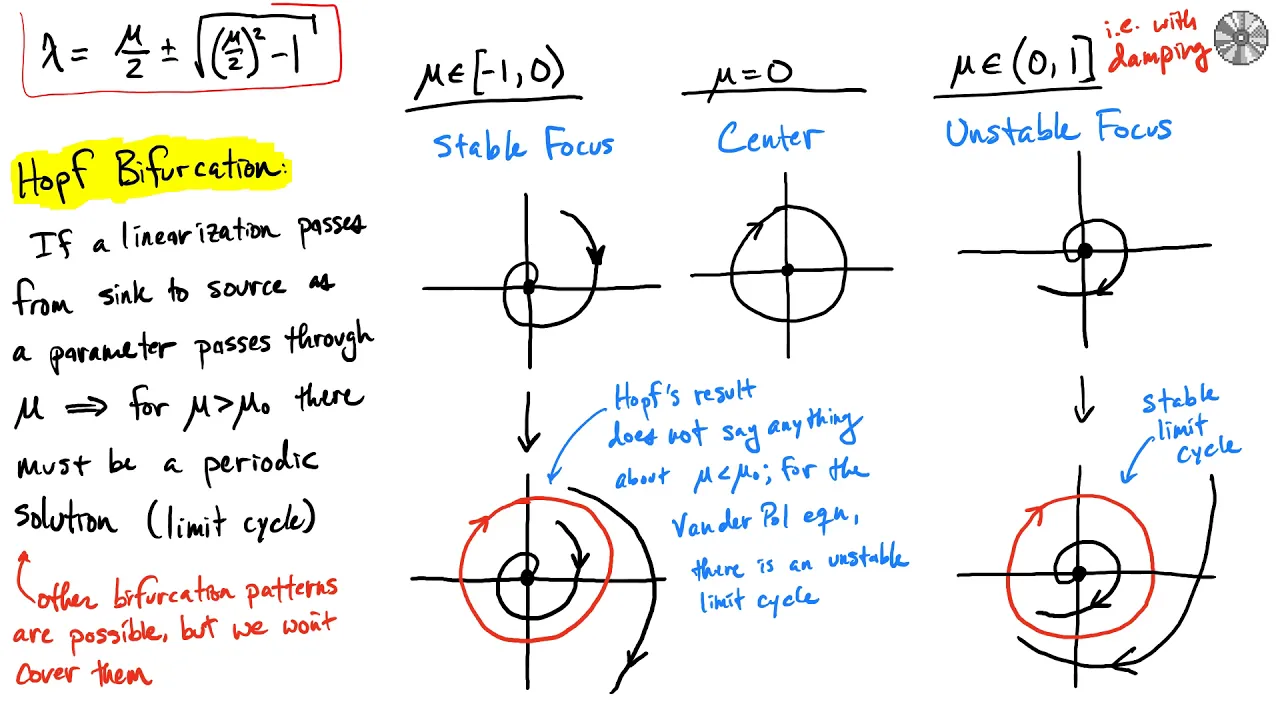
This lecture provides an accessible transition from standard linear systems to nonlinear behaviors. It defines limit cycles as isolated periodic orbits—a feature unique to nonlinear systems—and explains how they differ fundamentally from simple linear centers.

Why this video
This video focuses on the historical baseline for limit cycle research: the Van der Pol oscillator. Created by a Dutch electrical engineer studying early radio vacuum tubes, this model illustrates how state-dependent damping generates a stable limit cycle from an unstable origin.
Gap Recommendation: The physics of the Van der Pol oscillator can feel mathematically abstract on a blackboard. To see it in action, search YouTube for "Van der Pol oscillator phase portrait animation" or look up "Van der Pol oscillator Geogebra interactive plot" to manipulate the damping coefficient and watch the circular trajectory deform.
Knowledge Checkpoint
- What physical state does a "fixed point" represent in a dynamical system?
- How do you distinguish a stable fixed point (sink) from an unstable fixed point (source)?
- Why is a limit cycle considered "isolated," and how does it differ from the nested orbits of a simple harmonic oscillator?
- What is the real-world origin of the Van der Pol oscillator model?
Module 3: Bifurcation Theory: When Systems Mutate
Systems do not stay static; they change when external parameters vary. This morphing is called bifurcation theory. In this module, we explicitly split our study into discrete bifurcations (step-by-step maps where feedback paths create a cascading route to chaos) and continuous bifurcations (smooth physical systems where fixed points collide, trade stability, or trigger periodic behaviors).
Recommended Videos
Why this video
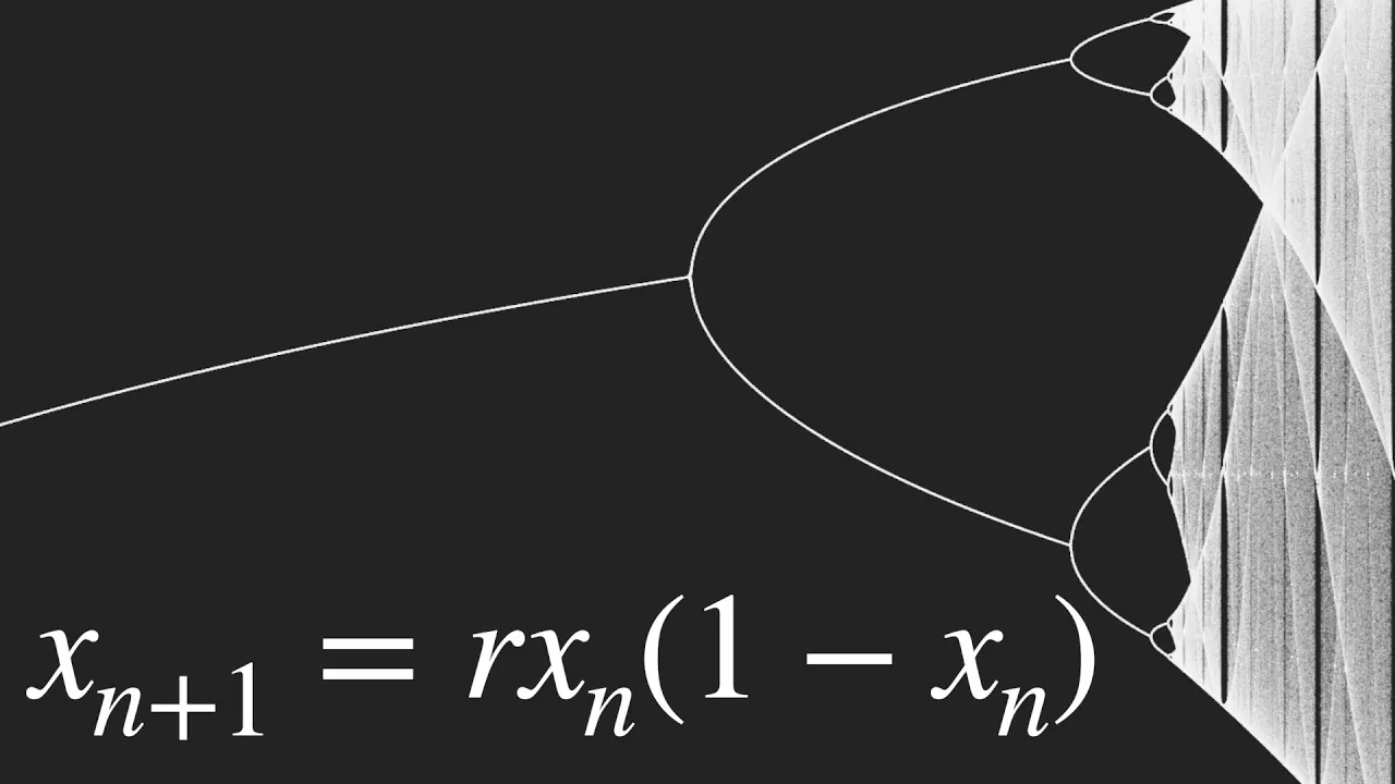
This is a masterpiece of science communication. It explains discrete bifurcations using the logistic map equation. You will watch a simple population growth model branch into two-period oscillations, then four, then eight—a classic "period-doubling cascade" that serves as a universal gateway to chaos.

Why this video
This lecture shows you what continuous bifurcations look like in 2D space. Using a simple model, it walks through a saddle-node bifurcation: the literal collision and mutual annihilation of a stable node and an unstable saddle point.

Why this video
This video explains the crucial Hopf bifurcation, which marks the birth of an oscillation. It links the mathematical transition—where a stable equilibrium point loses stability and births a limit cycle—to fluid dynamics, such as the real-world vortex shedding behind an obstacle.
Gap Recommendation: Continuous bifurcations (such as transcritical and pitchfork bifurcations) can look like dry algebra on static chalkboards. To grasp them geometrically, search YouTube for "transcritical bifurcation visual demonstration" or "pitchfork bifurcation animation".
Knowledge Checkpoint
- How does a discrete system (like the Logistic Map) transition from a single stable population to period-doubling oscillations?
- What physical event occurs during a 2D saddle-node bifurcation?
- What is a Hopf bifurcation, and how does it explain the sudden onset of physical oscillations (like fluid vortex shedding)?
- How do you distinguish between transcritical, pitchfork, and saddle-node bifurcations based on how their fixed points behave?
Module 4: The Strange World of Chaos & Attractors
When a continuous dynamical system has three or more dimensions and lacks linear stability, trajectories can be confined to a bounded region without ever repeating or crossing. This is chaos. Here, we analyze the famous Lorenz system, map the structure of "strange attractors," and explore the sensitive dependence on initial conditions known as the Butterfly Effect.
Recommended Videos
Why this video
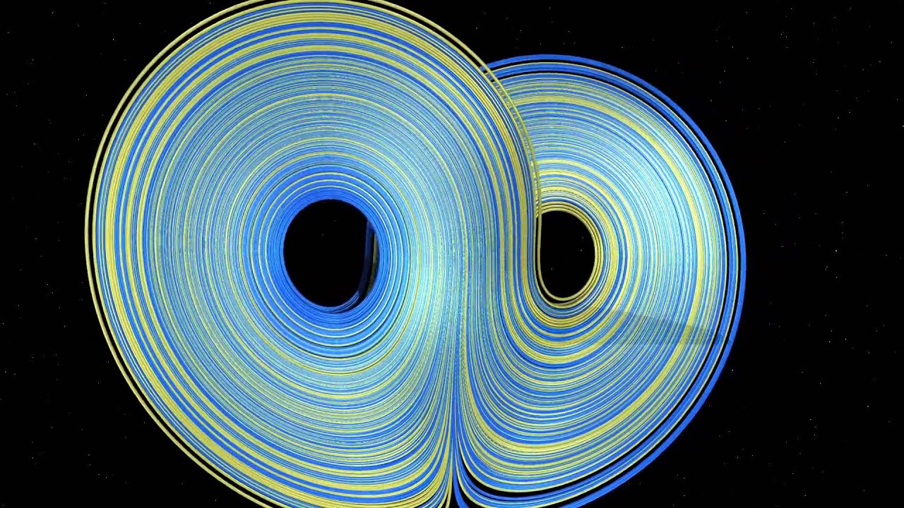
A gorgeously animated documentary chapter that explains Edward Lorenz’s weather model. It shows how simplifying atmospheric convection equations yielded a beautiful, butterfly-shaped coordinate trajectory: a strange attractor that is highly sensitive to initial conditions.
Why this video
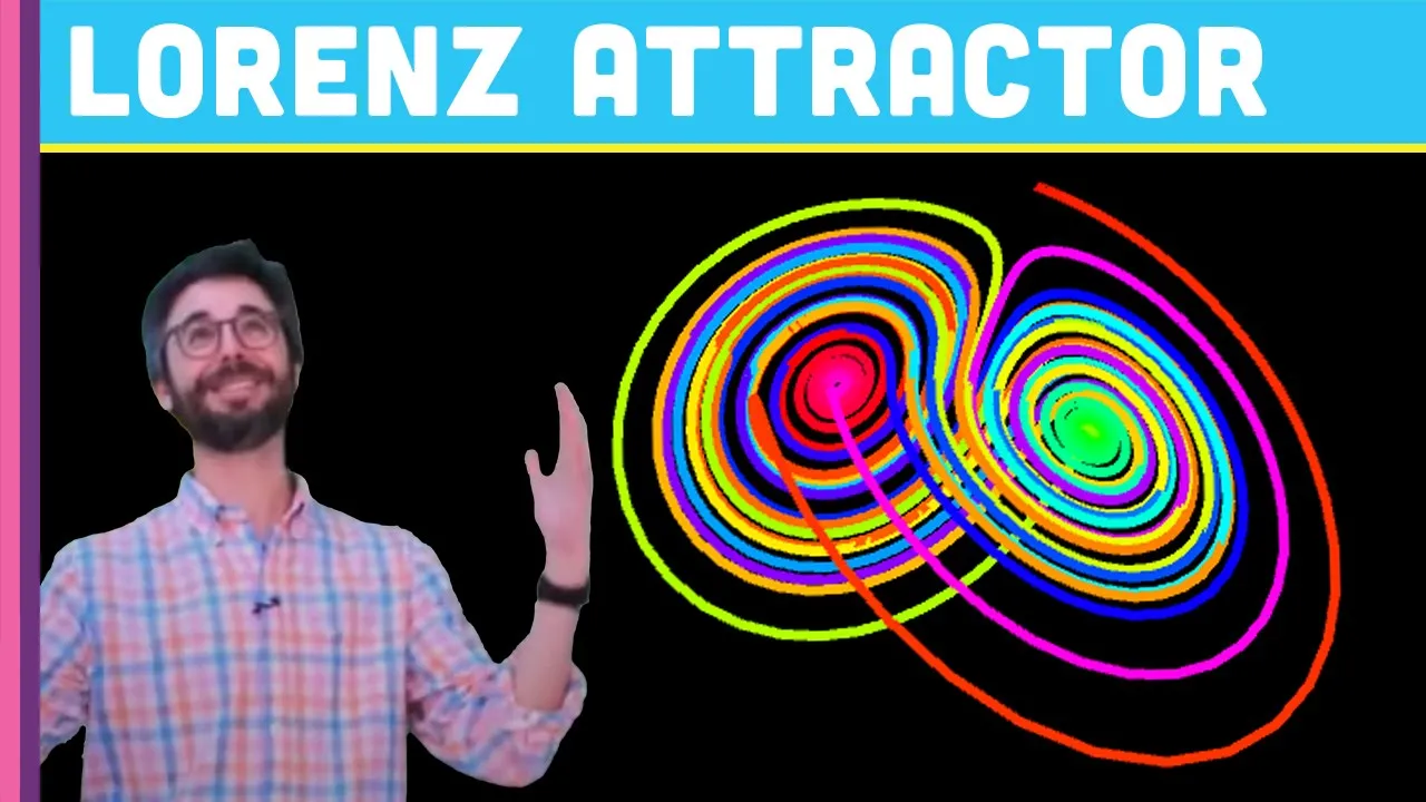
There is no better way to understand the Lorenz Attractor than to build it yourself. In this highly engaging video, you will see the three ordinary differential equations coded line-by-line, watching a chaotic 3D coordinate curve unfold on screen.

Why this video
This video explains the history and mathematics behind Lorenz's 1963 breakthrough. It breaks down how a deterministic, three-variable mathematical model destroyed the notion of long-term predictability in physics and weather forecasting.
Knowledge Checkpoint
- What are the three differential equations that govern the Lorenz system?
- Why does continuous chaos require a system to have at least three dimensions?
- What is the "Butterfly Effect," and why does it make long-term forecasting impossible even in entirely deterministic systems?
- What makes an attractor "strange" compared to a standard point attractor or a limit cycle?
Module 5: Fractal Geometry: The Infinite Dimensions
If you zoom into a strange attractor, you will find that its trajectories never overlap, meaning it has an infinite number of layers packed into a finite space. To measure this, we need fractal geometry. In this final module, we study self-similarity, calculate fractal dimensions, and explore how chaotic boundaries catalog beautiful structures like the Mandelbrot and Julia Sets.
Recommended Videos

Why this video
This highly produced, visually clear video explains the mathematics of the Mandelbrot set. It shows how iterating the simple complex function defines a boundary separating numbers that remain bounded from those that escape to infinity.

Why this video
This tutorial clarifies the deep connection between the Mandelbrot Set and Julia Sets. It explains how Mandelbrot serves as a visual catalog or map of all possible Julia Sets, determined by whether a given coordinate point yields a connected or disconnected Julia fractal.

Why this video
This video uncovers a surprising mathematical connection: how the constant appears naturally inside the Mandelbrot Set. By counting the number of iterations required to pass through the bottleneck near the cusp point (), it reveals the deep unity of mathematics.

Why this video
This video explains how to calculate a fractal dimension. Unlike traditional integer dimensions (1D lines, 2D planes), fractals occupy intermediate, fractional dimensions. This guide walks you through the scaling math that quantifies how much space these intricate shapes fill.
Knowledge Checkpoint
- What is the basic recursive formula used to generate the Mandelbrot set?
- How does the Mandelbrot set act as a visual catalog for connected and disconnected Julia sets?
- What is a fractal dimension, and how can an object have a dimension of 1.58?
- How does the concept of self-similarity manifest when zooming into the boundary of the Mandelbrot set?
Course Map
Key People Index
- Edward Lorenz (1917–2008): An American meteorologist and pioneer of chaos theory. He discovered the chaotic attractor that bears his name while modeling atmospheric convection, coining the term "Butterfly Effect."
- Steven Strogatz (1959–Present): An applied mathematician and Professor at Cornell University. His textbooks and public lectures popularized the geometric approach to teaching nonlinear dynamics and chaos.
- Balthasar van der Pol (1889–1959): A Dutch physicist and electrical engineer who initiated the study of experimental dynamics and limit cycles by modeling electrical oscillations in vacuum tubes.
- Benoit Mandelbrot (1924–2010): A Polish-born French-American mathematician who coined the term "fractal" and developed fractal geometry, demonstrating how rough, organic shapes in nature have mathematical order.
- Gaston Julia (1893–1978): A French mathematician who first investigated complex dynamic iterations by hand in the early 20th century, laying the foundation for modern computer-generated fractal geometry.
Final Self-Assessment
Complete this comprehensive checklist to verify your understanding of dynamical systems, chaos, and fractals:
- State Space Mastery: I can define a state space and visualize how a physical system maps to geometric coordinates.
- Vector Fields vs. Trajectories: I can look at a vector field and trace the likely path of a trajectory.
- Stability Classification: I can identify stable fixed points, unstable fixed points, and saddle points in a phase portrait.
- Limit Cycle Mechanisms: I can explain why limit cycles are unique to nonlinear systems and how the Van der Pol oscillator functions.
- Bifurcation Mechanics: I can describe what happens to fixed points during a saddle-node bifurcation.
- Discrete Chaos Path: I can explain how the period-doubling cascade in the Logistic Map leads to chaotic behavior.
- Dimensionality of Chaos: I understand why continuous chaotic attractors require a minimum of three dimensions.
- Defining Strange Attractors: I can explain why a strange attractor has infinite length but is bound to a finite volume.
- Mandelbrot Calculation: I can explain how the recursive equation is used to determine if a point is in the Mandelbrot set.
- Fractal Dimensions: I can calculate a simple fractal dimension (like the Sierpinski Triangle or Cantor Set) using scaling and self-similarity equations.